Neural Nets: Biological and Statistical Motivation #
Cognitive psychologists, neuroscientists, and others trying to understand complex information processing algorithms have long been inspired by the human brain.
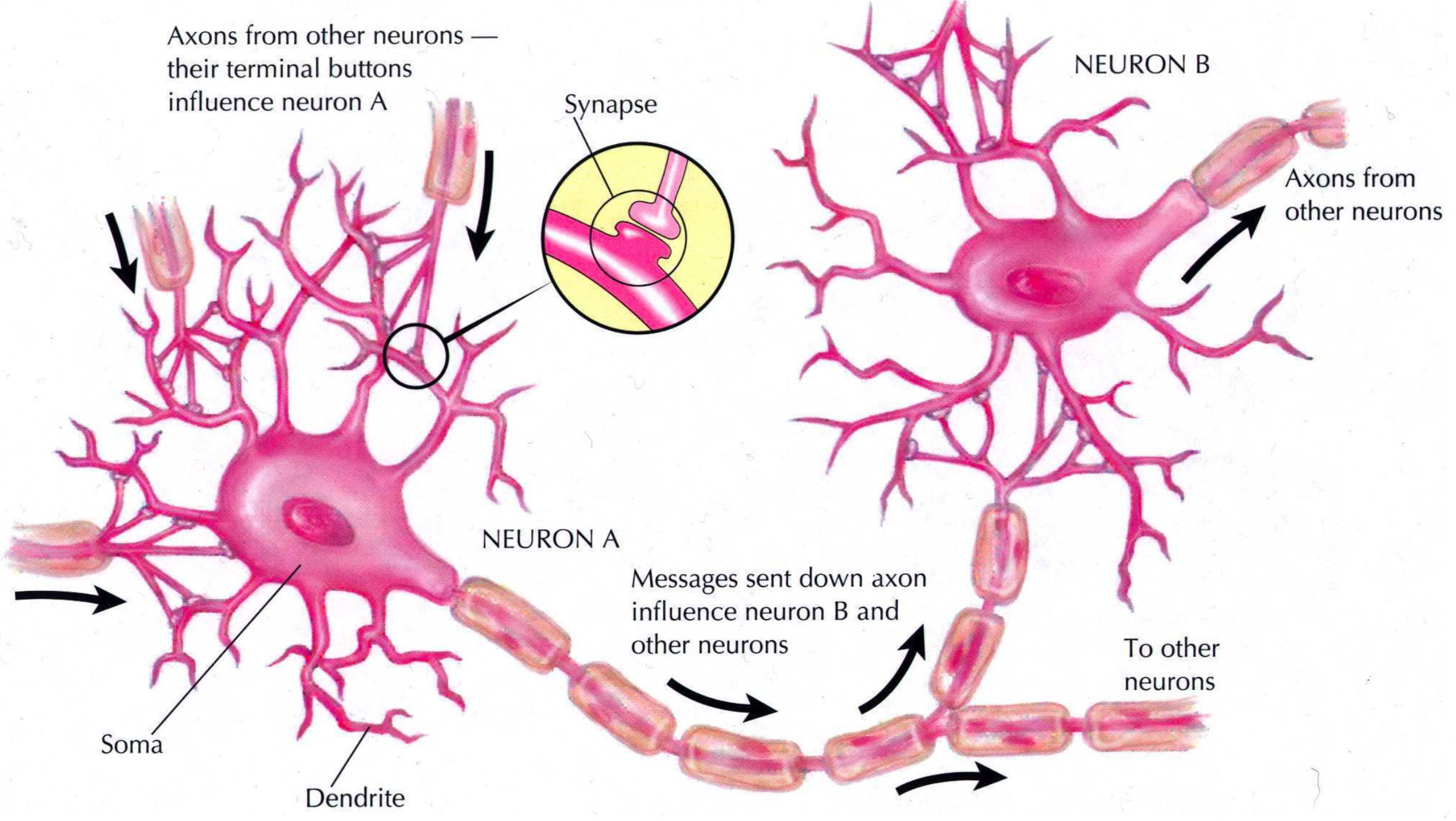
Figure 1: Image by David Plaut
The (real) picture is, not surprisingly, complicated. But a few key themes emerge:
- The firing of neurons produces an activation that flows through a network of neurons.
- Each neuron receives input from multiple other neurons and contributes output in turn to multiple other neurons.
- Local structures in the network can embody representations of particular semantic information, though information can be (and is) distributed throughout the network.
- The network can learn by changing the connections (and the strength of connections) among neurons.
Artificial Neural Networks #
An Artificial Neural Network is a computational model comprised of interconnected nodes that are inspired by biological neurons.
Artificial Neurons #
Attempts to capture some of the apparent power of biological neural networks in the brain led to various idealized, computational models of neurons. The most common models used today look like the following:
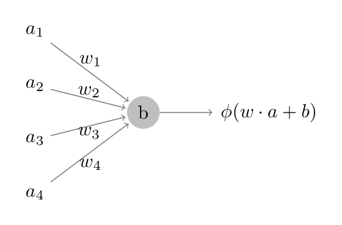
Here, the inputs to this neuron – the \(a_i\)’s – are the outputs from other neurons and are called activations.
The \(w_i\)’s on the edges describe the strength of these connections and are called the weights.
The output of the network is determined in three steps: (i) take a weighted sum of the activations \(w\cdot a\), (ii) shift it by a node-parameter \(b\), called a bias, and (iii) pass the result through a function \(\phi\), called the activation function (aka transfer function).
There are several different types of nodes, characterized by the form of the activation function \(\phi\).
- Linear
- \(\phi(z) = z\)
- Perceptron/Heaviside
- \(\phi(z) = 1_{(0,\infty)}(z)\).
- Sigmoidal
- \(\phi(z)\) is a sigmoidal (S-shaped) function,
that is smooth and bounded.
A common choice is the logistic function \[ \phi(z) = \frac{1}{1 + e^{-z}}, \] but the Gaussian cdf and a shifted and scaled version of \(\tanh\) are also used.
- Rectified Linear Unit (aka ReLU)
- \(\phi(z) = \max(z,0)\).
- Bias nodes
- always output 1
- Pass-through nodes
- \(\phi(z) = z\)
\(\cdots\)
Different kinds of nodes can be used and combined in any network.
Keep in mind that this neuron language is only a metaphor.
Networks #
We now combine these units into a computational network. This can be done in various ways, but today we will look at the most basic, a multi-layer feed-forward neural network (MLFFNN).
These networks are designed in layers, each comprised of one or more artificial neurons, or nodes.
-
The input layer takes in the data and usually consists of pass-through or purely linear nodes.
-
The output layer converts the computation into a form needed in how the network is used.
For two-class classification problems, for example, a single binary output node does the trick.
Another common example is to produce a probability distribution via the softmax combination. This takes the outputs \(z_1,\ldots,z_p\) of several output nodes and transforms the \(j^{\rm th}\) output to \[ \frac{e^{z_j}}{\sum_k e^{z_k}}. \]
In a regression problem, the output layer might be a single node that takes continuous values.
-
In between input and output are one or more hidden layers. A network with more than one hidden layer is often called a deep network.
As we will see, next week, some networks have additional filters (e.g., convolution) or tranformation (e.g., pooling) between layers.
Putting these layers together, a multi-layer feed-forward neural network looks like:
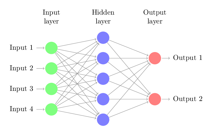
(For a fancier interactive visualization, see here.) These networks will be the focus of our study today.
The Statistical Problem #
A MLFFNN represents a parametrized function of its inputs, with parameters consisting of all the weights and biases. We can use these functions to fit complex data.
Such networks provide an efficiently trainable family that can approximate a broad class of functions.
A principle of universality indicates that a class of functions can be approximated arbitrarily well by a specified family of functions. MLFFNN’s have such a property.
For example:
-
An arbitrary (Borel measurable) real-valued function on the real numbers can be approximated arbitrary closely by the family of simple functions (finite, linear combination of indicators of measurable sets).
-
An arbitrary (computable) function can be approximated by a family of binary circuits comprised of NAND (not-and) gates.
Reflection 1 #
Construct a specific (e.g., including the weights and biases) single-hidden-layer network with one linear input, one linear output, and two perceptron hidden nodes that gives the indicator function of the interval \([1,2]\) (don’t worry about the endpoints).
If you modify your network to use sigmoidal nodes in the hidden layer (using, say, the logistic function), how well can you approximate the target function?
How does this result lead to a universality theorem for single-hidden layer, feed-forward neural nets? Roughly what does the theorem say?
Reflection 2 #
A (two-input) NAND gate is a binary function that takes two binary inputs and returns the complement of the inputs’ logical and.
| a | b | (NAND a b) |
|---|---|---|
| 0 | 0 | 1 |
| 0 | 1 | 1 |
| 1 | 0 | 1 |
| 1 | 1 | 0 |
Construct a single-node neural network with binary inputs that is equivalent to a NAND gate.
Optional Exercise (for later) #
Combine several NAND gates from Reflection 2 to construct a network with two binary inputs and two binary outputs that computes the binary sum of its inputs. (The two binary outputs corresponds to the two binary digits of the sum.) Hint: this network may have some connections within layer.
Exercise #
Design a data structure or class that represents a MLFFNN, along with a function to construct such a network with random Normal weights and biases.
For simplicity, you may assume that all nodes in each layer have the same type.
Keep this lightweight and brief; we will build on this as we go.
Start by thinking about what data you need: activation functions? number of nodes per layer? weights? biases? …
Mathematical Setup and Forward Propagation #
To do computations with these networks, it will be helpful to define the quantities involved carefully. In particular, we will express the computations in terms of matrices and vectors associated with each layer. This will not only make the equations easier to work with, but it will also enable us to use high-performance linear algebra algorithms in our calculations.
At layer \(\ell\) in the network, for \(\ell = 1,\ldots,L\), define:
- Number of nodes
- Let \(n_\ell\) be the number of nodes in the layer.
- Weight matrix
- \(W_\ell\), where \(W_{\ell,jk}\) is the weight from node \(j\) in layer \(\ell-1\) to node \(k\) in layer \(\ell\).
- Bias vector
- \(b_\ell\), where \(b_{\ell,j}\) is the bias parameter for node \(j\) in layer \(\ell\).
- Activation vector
- \(a_\ell\), where \(a_{\ell,j}\) is the activation produced by node \(j\) in layer \(\ell\). The input vector \(x\) is labeled \(a_0\).
- The weighted input vector
- \(z_\ell = W_\ell^T a_{\ell-1} + b_\ell\), which will be convenient for some calculations.
We thus have the recurrence relation:
\[\begin{aligned} a_\ell &= \phi(W_\ell^T a_{\ell-1} + b_\ell) \cr &= \phi(z_\ell) \cr a_0 &= x. \end{aligned}\]
for layers \(\ell = 1, \ldots, L\).
Question: What is \(W_1\) in the typical case where the input layer simply reads in one input value per node?
Activity #
Define a function forward(network, inputs, ...) that takes a network and a
vector of inputs and produces a vector of network outputs. Maybe this will be
a method on your network class.
Learning: Back Propagation and Stochastic Gradient Descent #
Our next goal is to help a neural network learn how to match the output of a desired function (empirical or otherwise).
In a typical supervised-learning situation, we train the network, fitting the model parameters \(\theta=(b_1,\ldots,b_L,W_1,\ldots,W_L)\), to minimize a cost function \(C(y,\theta)\) that compares expected outputs on some training sample \(\mathcal{T}\) of size \(n\) to the network’s predicted outputs.
In general, we will assume that \[ C(y,\theta) = \frac{1}{n} \sum_{x\in\mathcal{T}} C_x(y,\theta), \] where \(C_x\) is the cost function for that training sample. We also assume that the \(\theta\)-dependence of \(C(y,\theta)\) is only through \(a_L\).
But for now, we will consider a more specific case: \[ C(y,\theta) = \frac{1}{2 n} \sum_{x\in\mathcal{T}} \|y(x) - a^L(x, \theta)\|^2. \] There are other choices to consider in practice; an issue we will return to later.
Henceforth, we will treat the dependence of \(a^L\) on the weights and biases as implicit. Moreover, for the moment, we can ignore the sum over the training sample and consider a single point \(x\), treating \(x\) and \(y\) as fixed. (The extension to the full training sample will then be straightforward.) The cost function can then be written as \(C(\theta)\), which we want to minimize.
Interlude: Gradient Descent #
Suppose we have a real-valued function \(C(\theta)\) on a multi-dimensional parameter space that we would like to minimize.
For small enough changes in the parameter, we have \[ \begin{aligned} \Delta C &\approx \sum_k \frac{\partial C}{\partial \theta_k} \Delta\theta_k \cr &= \frac{\partial C}{\partial \theta} \cdot \Delta\theta, \end{aligned} \] where \(\Delta\theta\) is a vector \((\Delta\theta)_k = \Delta\theta_k\) and where \(\frac{\partial C}{\partial \theta} \equiv \nabla C\) is the gradient of \(C\) with respect to \(\theta\), a vector whose \(k^{\rm th}\) component is \(\frac{\partial C}{\partial \theta_k}\).
We would like to choose the \(\Delta\theta\) to reduce \(C\). If, for small \(\eta > 0\), we take \(\Delta\theta = -\eta \frac{\partial C}{\partial \theta}\), then \(\Delta C = -\eta \|\frac{\partial C}{\partial \theta}\|^2 \le 0\), as desired.
The gradient descent algorithm involves repeatedly taking \[\theta’ \leftarrow \theta - \eta \frac{\partial C}{\partial \theta}\] until the values of \(C\) converge. (We often want to adjust \(\eta\) along the way, typically reducing it as we get closer to convergence.)
This reduces \(C\) like a ball rolling down the surface of the function’s graph until the ball ends up in a local minimum. When we have a well-behaved function \(C\) or start close enough to the solution, we can find a global minimum as well.
For neural networks, the step-size parameter \(\eta\) is called the learning rate.
So, finding the partial derivative of our cost function \(C\) with respect to the weights and biases gives one approach neural network learning.
Unfortunately, this is costly because calculating the gradient requires calculating the cost function many times, each of which in turn requires a forward pass through the network. This tends to be slow.
Instead, we will consider an algorithm that computes all the partial derivatives we need using only one forward pass and one backward pass through the network. This method, back propagation, is much faster than naive gradient descent.
Back Propagation #
The core of the back propagation algorithm involves a recurrence relationship that lets us compute the gradient of \(C\). The derivation is relatively straightforward, but we will not derive these equations today. A nice development is given here if you’d like to see it, which motivates the form below.
At a high level, think of back propagation as a fancy way to do the chain rule. A neural network, after all, is just a bunch of composed functions: we apply an activation function to the output from another activation function that was applied to another activation function… and if we know the derivative of the activation function, we can use the chain rule to calculate the derivative of everything at the same time as we calculate the output of the function.
Back propagation is a special case of automatic differentiation, a general technique for getting exact derivatives of functions. Back propagation is a useful variety that gets the derivative of the function with respect to every parameter all at once, using only one extra pass through the neural network.
To start, we will define two specialized products. First, the Hadamard product of two vectors (or matrices) of the same dimension is the elementwise product, \((u \star v)_i = u_i v_i\) (and similarly for matrices).
Second, the outer product of two vectors, \(u \odot v = u v^T\), is the matrix with \(i,j\) element \(u_i v_j\).
We will also assume that the activation function \(\phi\) and its derivative \(\phi’\) are vectorized.
Also, it will be helpful to define the intermediate values \(\delta_{\ell,j} = \frac{\partial C}{\partial z_{\ell,j}}\), where \(z_\ell\) is the weighted input vector. Having the vectors \(\delta_\ell\) makes the main equations easier to express.
The four main backpropagation equations are:
\[\begin{aligned} \delta_{L} &= \frac{\partial C}{\partial a_L} \star \phi’(z_L) \cr &= (y - a_L(x)) \star \phi’(z_L) \cr \delta_{\ell-1} &= (W_\ell \delta_\ell) \star \phi’(z_{\ell-1})\cr \frac{\partial C}{\partial b_\ell} &= \delta_\ell \cr \frac{\partial C}{\partial W_\ell} &= a_{\ell-1} \delta_\ell^T. \end{aligned}\]
For the last two equations, note that the gradients with respect to a vector or matrix are vectors or matrices of the same shape (with corresponding elements, i.e., \(\partial C/\partial W_{\ell,jk} = a_{\ell-1,j} \delta_{\ell,k}\)).
In the back propagation algorithm, we think of \(\delta_L\) as a measure of output error. For our mean-squared error cost function, it is just a scaled residual. We propagate this error backward through the network via the recurrence relation above to find all the gradients.
The algorithm is as follows:
-
Initialize. Set \(a_0 = x\), the input to the network.
-
Feed forward. Find \(a_L\) by the recurrence \(a_{\ell} = \phi(W_\ell^T a_{\ell-1} + b_\ell)\).
-
Compute the Output Error. Initialize the backward steps by computing \(\delta_L\) using equation (1).
-
Back Propagate Error. Compute successive \(\delta_\ell\) for \(L-1,\ldots,1\) by the recursion (2).
-
Compute Gradient. Gather the gradients with respect to each layer’s weights, biases via equations (3) and (4).
While we have used the same symbol \(\phi\) for the activation function in each layer, the equations and algorithm above allow for \(\phi\) to differ across layers.
Above we computed the gradient of a loss function based on a single sample. But given any training sample, the resulting loss function and corresponding gradients are just the average of what we get for a single training point. (Equations 1-4 work in both cases.)
We can now use the gradients from backward propagation for gradient descent. But there is a more efficient approach to the same goal…
Stochastic Gradient Descent #
In practice, using the entire training sample (which may be quite large) to compute each gradient is wasteful. We can in fact approximate the gradient over the entire training set with only a subset, such as a random sample or even a single instance. This approximation is called stochastic gradient descent.
In practice, this is usually done as follows:
-
Training proceeds in a series of epochs, each of which comprises a pass through the entire training set.
-
During an epoch, the training set is divided into non-overlapping subsets, called mini-batches, each of which is used in a pass of stochastic gradient descent.
-
After each epoch, the training set is randomly shuffled, so that the mini-batches used across epochs are different.
-
Across epochs, the learning rate is adjusted, either adaptively or according to a reduction schedule.
-
Before training, the network is usually initialized with random weights and biases.
Pseudo-code:
0. Select initial values for the parameters theta. This is
   often done by choosing them randomly.

   Initialize the learning rate \eta and the
   schedule for changing it as the algorithm proceeds.

1. Until stopping conditions are met, do:

   a. Shuffle the training set and divide into m mini-batches
      of designated size.

   b. For b = 1, ..., m, set

      theta = theta - eta * gradient(C_b(theta))

      where C_b is the cost function for mini-batch b

   c. Make any scheduled adjustments to the learning rate
What’s Deep about Deep Learning? #
Deep learning is the buzzword of the moment, and an enormous amount of attention is focused on applying and developing them.
We call a multi-layer network deep if it has more than one hidden layer, and commonly used models have hundreds of layers.
We’ve seen that single-hidden-layer FF neural networks can approximate arbitrarily complicated functions, if given enough nodes.
-
What would we gain or lose by having more hidden layers?
-
Is there a qualitative difference between say 2-10 hidden layers and 1000, if we control for the total number of model parameters?
-
And if we do use more hidden layers, what effect will this have on training?
-
Will backpropagation with stochastic gradient descent still work? Will it still be efficient? If not, how should we train these networks.
-
Are there useful network designs beyond feed-forward networks?
The Benefits of Depth #
Think of any complicated system – your laptop, your car, a nuclear reactor – it is composed of many interconnected modules, each serving a focal purpose.
Take the computer as an example. In principle, we can arrange all the circuitry in your laptop in a single layer of logic gates. (Such a layer of binary circuits has a universality property and can compute any computable function.)
But such an arrangement is harder in several ways, including:
- It is hard to design.
- It is hard to understand its function given it’s inputs and outputs.
- It requires many more gates/elements than a more modular design.
Consider for example how much easier it is to create a binary adder with multiple layers. Even for a simple task like computing the parity of a binary string requires exponentially more elements in a shallow circuit than a deep circuit.
This is a useful analogy for the benefits of depth in neural network models. Deep networks:
- Are easier to design.
- Generate intermediate representations of the inputs that make it easier (though not easy) to understand the networks function.
- Require many fewer nodes than a shallow network of comparable power.
Of course, these benefits are not without costs. Most notably: deep networks can be hard to train.
Training Deep Networks is Hard #
Consider the “Hello, World” of neural networks: the MNIST hand-written digits, a collection of 70,000 \(28\times 28\) images.
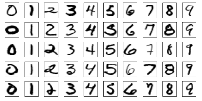
A network to recognize these digits might have 784 inputs (one per pixel) and 10 outputs (one per digit).
Fitting this with a standard feed forward network and SGD on half the data gives 97% correct classification with one hidden layer, almost 96% with two hidden layers, and the rate drops a bit and oscillates in the same range as the number of layers increases. Depth is not helping.
We can look at how the parameters are changing in the network during fitting, and it reveals a key fact: for any number of hidden layers, the earlier layers change more slowly than the later layers. The problem gets worse as we add more layers.
This is called the vanishing gradient problem. A dual issue – called the exploding gradient problem can also occur. In either case, the underlying problem is the instability of the gradient in deep networks.
One reason this happens is because the gradients of \(\frac{\partial C}{\partial \theta}\) depend on a product across layers of terms that can vary substantially in magnitude.
Unstable gradients are just one challenge to training. Others include multi-modality and the sensitivity of performance to tuning parameters.
Tricks of the Trade #
Faster Optimizations #
The venerable gradient descent algorithm moves generally downhill towards a (local) minimum of the cost function \[\theta’ \leftarrow \theta - \eta \frac{\partial C}{\partial \theta}.\] But this can produce several problems: going slowly in steep valleys, getting stuck in local minima, moving over a valley, et cetera..
Momentum #
Gradient descent has no memory. Instead, maintain an exponentially-weighted running average of the gradient and accumulate these. \[\begin{aligned} m &\leftarrow \beta m - \eta\nabla C(\theta + \beta m) \cr \theta &\leftarrow \theta + m \end{aligned}\] (This is Nesterov momentum, which is commonly used.) The β parameter is (inversely) related to “friction” in the movement of the parameter. This tends to move significantly faster than gradient descent alone, by roughly a factor of \(1/(1 + \beta)\).
Adaptive #
Adaptive optimization algorithms like ADAM combine the ideas of momentum with a dynamic transformation that speeds up the motion on the edge of flat valleys. This requires tuning of several hyperparameters and is easy to get wrong. But when it is suitable, it allegedly perfoms well.
Regularization #
Smoothing the cost function. Just like regularization in linear models, we can add a penalty term to the weight matrix, penalizing having large weights. This works just like regularization in other models, because it encourages the model not to overfit by picking weird weights.
Dropout #
A simple, interesting, and effective regularization technique is called dropout (see the original paper here), where randomly selected nodes are ignored during training. During each step of training, each node (excluding output nodes) is completely ignored during that step with probability \(p\). After training, outputs are scaled by a factor \(1-p\) to stay in the training range.
That is, their activations are excluded from the forward propogation, and the any weight/bias updates during the backward propogation are not applied. This has the effect of making the network’s output less sensitive to the parameters for any node, reducing overfitting and improving generalizability.
Data Augmentation #
Transfer Learning #
Learning from previously trained models
New Layer Types #
The networks we have seen so far are fully connected: each node transmits its output to the inputs of all nodes in the next layer. And all of these edges (and nodes) have their own weights (and biases).
But for many kinds of data – especially images and text – new architectures turn out to be useful, even essential.
Current approaches to building deep learning models focus on combining and tuning layers of different types in a way that is adapted to the data, the outputs, and the types of internal representations that might perform well for the task.
Convolutional Layers/Networks #
Convolutional neural networks mimic the structure of the human visual system, which uses a complex hierarchy of decomposition and recombination to process complex visual scenes quickly and effectively.
Recall: one dimensional convolution \[ (a \star f)_k = \sum_j f_j a_{k-j} \] This generalizes to multiple dimensions and inspires the filtering steps to be used below.
The key ideas behind convolutional neural networks are:
- Visual fields as inputs and local receptive fields for modes
- Capturing multiple features through sub-layers of the hidden layer, usually called feature maps.
- Shared parameters within each sublayer (feature map).
- Pooling – dimension reduction
Local Receptive Fields #
   Input layer                  A Feature Map
                                within Hidden Layer
........................
........................
........................
........................           . . .
........................           . . .
........................           . . .
........................
........................
........................
........................
........................
........................
Key parameters:
- Filter size (size of local receptive field)
- Stride (how much filter is shifted)
This structure is repeated for each sub-layer (feature map) in the hidden layer.
Shared Weights and Biases #
Each sub-layer (feature map) in the hidden layer shares the same weights and biases: \[ a_{\ell m,jk} = \phi\left( b_m + \sum_r \sum_s W_{\ell m, rs} a_{\ell - 1, j+r, k+s} \right) \] where \(a_{\ell m, jk}\) is the output activation of node \((j,k\)) in feature map \(m\) in layer \(\ell\), \(W_{\ell m}\) is the matrix of weights that captures the local receptive field – which is sometimes called the filter, and \(a_{\ell - 1}\) is the matrix of activations from the previous layer.
Do you notice the convolution here? We can write this as \[ a_{\ell m} = \phi(b + W_{\ell m} \star a_{\ell-1}). \]
Because of this sharing, all the hidden neurons in a given feature map detect the same feature but at different parts of the visual field. A combination of feature maps thus decomposes an input image into a meaningful intermediate representation.
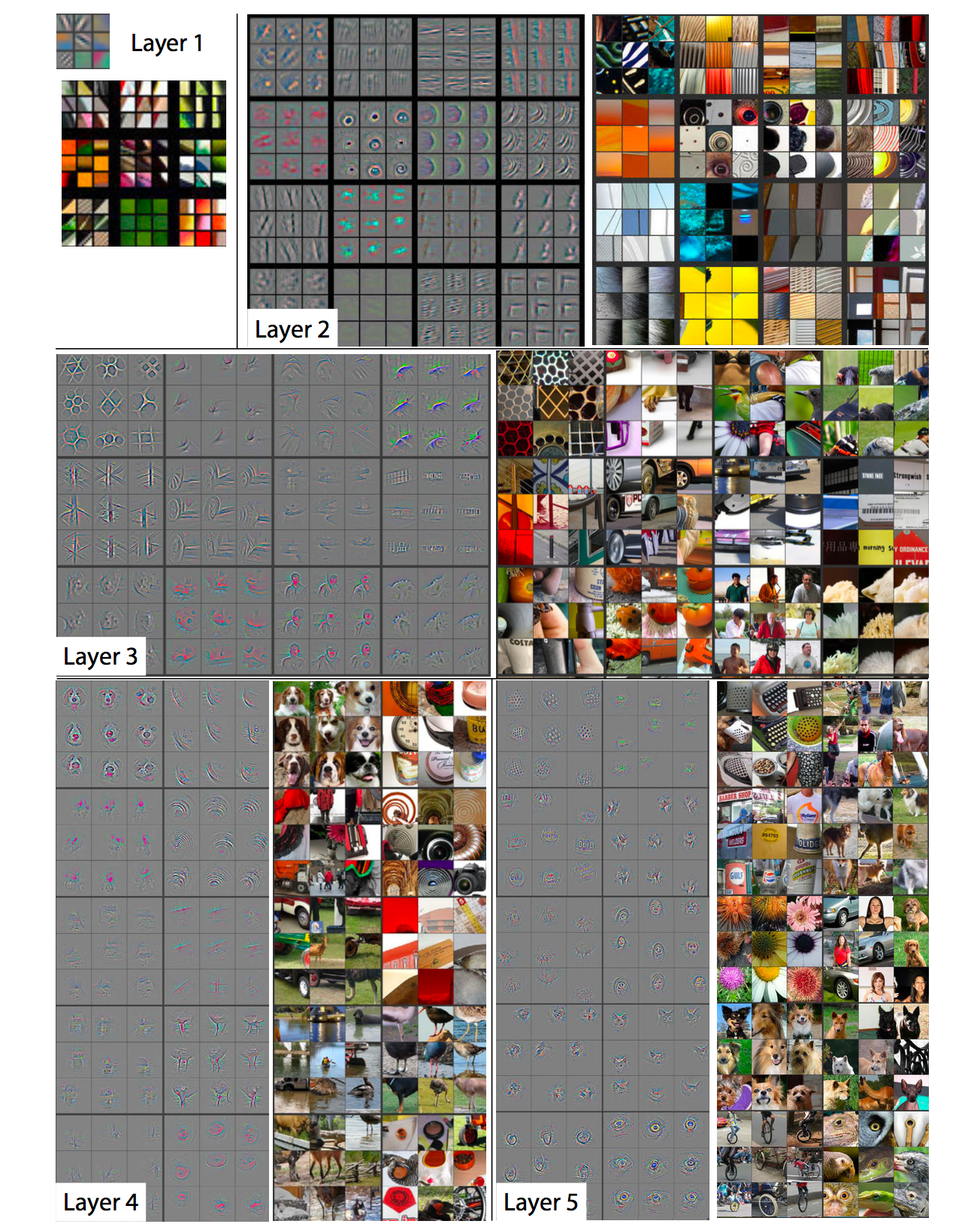
The following picture shows the layers of a fully-trained convolutional network from Zeiler and Fergus (2013) (paper here).
Pooling Layers #
A pooling layer in the convolutional network is designed to compress the information in the feature map, primarily as a form of dimension reduction. This is a layer without weights and biases, though it may have a tuning parameter that specifies how much compression is done.
Pooling operates on output of the nodes in a feature map, producing a feature map with fewer nodes.
Feature map output         Pooled Feature map

1 1 2 2 . . . .
1 1 2 2 . . . .
. . 3 3 . . . .              1 2 . .
. . 3 3 . . . .              . 3 . .
. . . . . . . .              . . . .
. . . . . . . .              . . . 4
. . . . . . 4 4
. . . . . . 4 4
Examples:
-
Max pooling – groups of nodes are reduced to one by taking the maximum of their output activations as the activation of the resulting node.
-
\(\mathcal{\ell}^2\) pooling – groups of nodes are reduced to one by taking the root-mean-square (\(\mathcal{\ell}^2\) norm) of their output activations.
Sample Network #
- Input layer (32 \(\times\) 32)
- Convolutional (4 \(\times\) 16 \(\times\) 16)
- 4 \(\times\) 4 local receptive fields
- Stride 2
- Four feature maps
- Max pooling (4 \(\times\) 4 \(\times\) 4)
- 4 \(\times\) 4 blocks
- Fully-connected output layer
The backpropogation equations can be generalized to convolutional networks and applied here. In this case, dropout would typically be applied only to the fully connected layer.
A few common tricks for training:
- Use rectified linear units (\(\phi(x) = \max(x,0)\)) in place of sigmoidal units.
- Add some small regularization (like a ridge term) to the loss function
- “Expand” the training data in various ways For example, with images, the training images can be shifted randomly several times by one or a few pixels in each (or random) directions.
- Use an ensemble of networks for classification problems
For a more detailed example, see this interactive visualization.
Softmax Layers #
The softmax function is a mapping from $n$-vectors to a discrete probability distribution on \(1\ldots n\):
\[ \psi_i(z) = \frac{e^{z_i}}{\sum_j e^{z_j}} \]
(Q: Why is this giving a probability distribution? What inputs give a probability of 1 for selecting 3?)
A softmax output layer in a neural network allows us to compute probability distributions.
If the output layer has \(n\) nodes, we obtain \[ a_{L,j} = \psi_j(z_L), \] where \(z_L\) is the weighted input vector in the last layer.
Other Types of Networks #
Recurrent Networks #
Adding memory and time.
Autoencoders #
Finding efficient representations of a data set.
Deep Learning Frameworks #
-
TensorFlow (C++, Python, Java)
Popular and powerful. Python/Numpy is main interface. Other languages exists but are still catching up.
Computational graph abstraction Good for RNNs
-
MXNET (C++, Python, R, JVM:Clojure/Scala/Java)
Easy structure, many languages, easy to extend, well supported and actively developed
-
DeepLearning4j (JVM)
Works with JVM languages, actively developed, increasing capabilities
-
Keras (High Level Wrapper for Python)
Provides a higher-level interface to use TensorFlow, with many pre-made layer types that can be easily fit together
-
Caffe (Python, C++/CUDA)
Can specify declaratively (less coding). Good for feedforward, tools for tuning. Good Python interface. Primarily for convolutional networks
-
Torch/PyTorch (Lua, C++/Python)
Modular, third-party packages, easy to read code, pretrained models
More coding, not great for RNNs
-
Microsoft Cognitive Toolkit/CNTK (C++, Python)
Model Zoos #
VGG. LeNet-*, AlexNet, ResNet, GoogLeNet, …