A data structure is a formal organization of data that supports a pre-specified set of operations on it, designed to allow efficient access and manipulation of the data it contains.
Most data structures are instantiated and maintained in main memory during the execution of a program, but some are designed to be work efficiently with external storage.
Data structures mesh closely with algorithms. Algorithms operate on data structures to produce their results, and the choices of data structure and algorithm can have a dramatic effect on the efficiency of a computation.
The most important feature that guides our choice of data structures is if a particularly representation allows us to efficiently compute the answers we need for our problem.
Aside on Computational Complexity #
We often have a choice of several data structures and algorithms to solve a problem. How can we understand and compare our choices?
Computer scientists use “big O notation” for as a tool for the analysis of algorithms. The basic premises are these:
- Every basic operation performed by a computer (e.g. addition, multiplication, comparison, etc.) takes the same amount of time.
- An algorithm is composed of many of these operations.
- The number of these operations executed for any given input depends on the size of the input, n.
It would be impractical to count every operation performed by a given algorithm – this would depend on the specific implementation, the programming language used, optimizations performed by the compiler or interpreter, and so on, and would hence be nearly impossible to find out.
Instead, big O notation captures the order of the relationship between n and the number of operations.
Mathematically, say g(n) is the number of operations performed by a specific algorithm on an input of size n. We say the algorithm is O(f(n)) iff a constant multiple of f(n) is an upper bound of g(n) for n sufficiently large.
Typically we simplify f(n) by dropping lower-order terms and constants.
There are related notations, such as “big Omega” notation, which gives a lower bound to the growth of the number of operations, and “big theta”, which says a function is bounded above and below by a function of the same order.
The purpose here is to focus on the algorithm itself, not its implementation in whatever programming language we’ve chosen. How fast is the algorithm given different size inputs, regardless of whether we implemented it on a fast computer or a slow programming language or with the world’s stupidest code? Different algorithms have different intrinsic performance, and choosing the right algorithm is the first step in the process of optimizing your code.
Examples:
- Computing the mean of a length \(n\) vector is an \(O(n)\) operation.
- Computing the pairwise distances for a set of \(n\) points is an \(O(n^2)\) operation.
- Computing all permutations of a string of length \(n\) is an \(O(n!)\) operation.
Algorithms and Data Structures are Important #
R users hold unusual beliefs about performance and optimization. If code can be written as matrix and vector operations, or in terms of a base function that’s implemented in C, it’s fast, so we figure out how to write all our algorithms to use vectorized base functions. If we can’t, we declare “Loops are slow in R, so I’ll write it in C++” and pull out the Rcpp package.
But as we will see with divide-and-conquer and dynamic programming algorithms, the choice of algorithm can make an enormous difference in speed. The difference between C and R isn’t nearly as big as the difference between an \(O(n)\) and \(O(n^2)\) algorithm.
Choice of data structures can make a similarly important difference. We must choose a structure that efficiently supports the operations we need for our problem.
Data Types #
A data type (or type for short) is a classification of data (usually in a programming language) that specifies to a compiler or interpreter how the data is to be stored and which operations can be legally performed on it.
Programming languages support a variety of data types. These are the basic ingredients we use in the data structures we will see below.
Primitive Types #
These represent data that are stored in a format that is (or is close to one) supported natively by the hardware and that have direct support as types in a programming language.
| Boolean | true, false |
|---|---|
| Integer | signed or unsigned integers in various ranges |
| Numeric | fixed precision floating point numbers |
| Character | represents a single glyph, various representations |
| Pointer | an address in memory |
There are others (e.g., fixed-width numbers, rational numbers, complex numbers) but these are the most commonly supported.
Examples #
In C++, each variable must be declared to be of a certain type; primitive types have reserved words to describe them:
bool            b;
char            c;
unsigned short  j = 32000;
int             i;
long            u = 1000000;
double          x = 1.24e-4;
int*            p;

b = true;
c = 'A';
i = 1024;
p = &i;  // address of i
In languages like Python or R, data types are not typically specified by the programmer but are inferred implicitly.
a = 24
b = 24.2
c = True
Aggregate Types #
These represent simple collections of values (of specified types) stored in a contiguous block of memory. They are building blocks in many more complex data structures.
| Tuple | fixed-length sequence of values, with each element having a specified type |
|---|---|
| Array | contiguous, fixed-length collection of values all of the same type |
| Record/Struct | structured group of named attributes of various types in contiguous storage |
| Union | region of memory that can store several specified types (sometimes tagged) |
In Python, we have tuples that look like (4, 'Hello', True) or (17.4, -32.3).
In C++, we specify records (called structs) with explicit types:
struct node {
    string        name;
    double        value;
    struct node*  next;
};
Object Types #
Most programming languages offer a facility for defining more complicated types, which store data and have certain behaviors.
| String | A sequence of characters |
|---|---|
| Enumeration | A value that can take only one |
| Function | A callable object; that is, a … function |
| File | A representation of a file in a file system |
| Stream | A stream of data elements made available sequentially |
| BigNum | An arbitrary-precision number |
| Object | A general type encapsulating specific data and behaviors |
We’ll talk more about creating objects and object-oriented programming in a few weeks.
Linked Data: References and Pointers #
A fundamental and oft-recurring feature of many data structures is that there are links from piece of data pointing to another piece of data in the same structure.
These links can take many forms from integers representing indices in some contiguous array, to hash keys, to pointers to specific memory locations (containing other records or data), and even to external data sources.
It’s worth keeping in mind that in many languages, variables representing complex data types are actually references (pointers) to the data. Consider this from Python. What happens?
a = [1, 2, 3, 4]
b = a
b[2] = 20
print(a)
Similarly, in a language like Java:
String s = "foo bar zap";
Here s is an object representing data encapsulated with various
behaviors/operations that are pre-specified. But the variable
s actually stores a pointer to the data itself.
This is in contrast with R which has no simple reference type. In R, we have:
a <- c(1, 2, 3, 4)
b <- a
b[3] <- 20

a
In Python, variable names point to locations in memory where data is stored, and multiple names can refer to the same location; in R, multiple names mean multiple versions of the data.
This fact can make it challenging (and or inefficient in time or memory) to create complex data structures in R. Moreover, large structures like arrays in R are copy on write, which can get costly.
One solution is to use environments, which can associate names with persistent data, kept as references. This is the idea behind Reference Classes in R.
Core Data Structures #
Data structures can be defined in the abstract through the set of operations they support and the requirements placed on the computational complexity of these operations.
More concretely, data structures can be defined through a specific implementation of these operations. The abstract representation of a data structure can have several distinct concrete implementations.
Here is a brief survey of some of the most commonly used data structures.
(Note: the abstract specification of data structures are sometimes called “abstract types”.)
Lists #
A list is linear, finite sequence of values.
Abstract specification:
head(L)returns first element of the listLin O(1) time.tail(L)returns the rest of the listLin O(1) time.cons(L, v)adds valuevto the head of the listLin O(1) time.
Implementations:
-
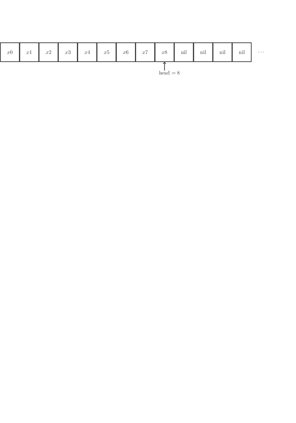
Arrays:
Store list items (or references) in array in reverse order, maintaining index to head, expand the array (by copying into a larger space) as needed.
-
Linked List:
Each item is a record with data and a pointer to next item (or nil if none).

-
Doubly-Linked List
Each item is a record with data and pointers to next and previous items (or nil if none).

Question #
Does R’s list data type match this description?
Stacks, Queues, Deques #
A stack is a collection of values where only the most recently added item is available. Items are available Last In, First Out (LIFO). (Think of a stack of cafeteria trays.)
Abstract specification:
push(S, x)adds itemxto the top of stackSin O(1) time.pop(S)removes and returns the top item on stackSin O(1) time. (Popping an empty stack is an error.)isEmpty(S)indicates whether stackSis empty in O(1) time.- (Optional)
peek(S)returns the top item on stackSwithout removing it, in O(1) time.
Implementations: Array or Linked List
A queue is a collection of values where only the least recently added item is available (at the front) and where items can be added only at the end. Items are available First In, First Out (FIFO). (Think of a line at the grocery store.)
Abstract specification:
enqueue(Q, x)adds itemxto the end of queueQin O(1) time.dequeue(Q)removes and returns the item at the front of queueQin O(1) time. (Dequeueing an empty queue is an error.)isEmpty(Q)indicates whether stackQis empty in O(1) time.- (Optional)
peek(Q)returns the top item on queueQwithout removing it, in O(1) time.
Implementations: Doubly-Linked List or Rolling Array
A deque (pronounced “deck”) is a generalization of stacks and queues that stands for double-ended queue.
The abstract specification states that items can be added to or
removed from either end in O(1) time, with operations addFront(D,x),
popFront(D), addRear(D,x), popRear(D), and isEmpty(D) at least.
Implementation is often with a doubly-linked list.
Language implementations:
collections.dequein Pythoncollections,rstackdeque, ordequerpackages in R (don’t useliqueueR)std::stackandstd::queuein C++DataStructures.jlfor Julia
Question #
Suppose you’ve written a program to scrape Wikipedia and extract data. It starts at a specific article and extracts all the links from that page. It then puts all those links on a stack.
To decide which article to look at next, it pops the top of the stack and loads that article, then puts all of its links onto the stack.
Describe the order in which it will visit the articles. At what point will it have visited all the links from the first article visited?
Priority Queues #
A priority queue is a collection of items with associated scores (called priorities) in which it is efficient to remove (or view) the item with highest priority. (Think of the line at a hospital emergency room, where the most serious cases are taken first.)
Abstract specification:
insert(Q, x, p)adds itemxwith prioritypto priority queueQ.removeHighest(Q)removes and returns the highest priority item from priority queueQ. (It is an error to remove from an empty queue.)findHighest(Q)returns highest priority item from priority queueQwithout removing it.isEmpty(Q)indicates whetherQis empty.
insert and findHighest can be implemented in O(1) time, though
for naive implementations the latter can be O(n).
Implementations: arrays, heaps
Language implementations:
heapqin Python standard library- In
heapq, you don’t specify a separate priority: items are sorted by their own value, not by a separate priority. But there’s a trick: If you make a tuple(priority, value), the<operator for tuples compares the first element first, then the second, and so on; so(1, "foo") < (2, "bar"). You can use this to insert items with any priority you want. - Note that if there is a tie, such as
(1, "foo") < (2, "bar"), Python compares the second element in the tuple. If the second element is a type that<is not defined for, this won’t work; you might need some way of breaking ties.
- In
collectionspackage in R
Question #
How could I use a priority queue to sort a bunch of items?
Hash Tables #
A hash table (aka dictionary, associative array, hash map, or sometimes map) that map (typically sparse) values of one type to values of another. We look up values stored in the table by their keys. Think of a dictionary: we look up the definition of a word using the word as a key into the dictionary.
Abstract specification (basic):
insert(H, k, v)– Insert valuevinto hash tableHassociated with keyklookup(H, k)– Find the value, if any, inHassociated with keykremove(H, k)– Remove a key and its associated value from the table- …
The idea is that these operations are fast, ideally O(1), even though the set of possible values may be large and sparse.
The trick to making this work is using a good hash function. A hash function is a function which takes an object (integer, tuple, string, anything) and returns a number. Hash functions are designed to be very fast, and so that slightly different inputs give very different outputs. The key property:
Two unequal objects are unlikely to have the same hash value
We will talk more about hash functions and their many uses later in the course.
Language Implementations:
- Native:
dictin python,mapin clojure, tables inlua, Julia, …. std::unordered_mapin C++collectionsorhashpackages in R (only string keys supported). R’s lists are not hash tables, and have O(n) lookup or worse. R does use hash tables internally (“environments”) to connect variable names to their values.
Here is a basic implementation of a hash table. Suppose a hash function gives output in the range [0, N], where N is a suitably large number. We pick a smaller number M and allocate an array of size M.
To add an item to the set, we calculate i = hash(item) mod M. Then look up the ith element in the array.
- If it is empty, add the item as the first element of a linked list.
- If it already contains an entry, search the linked list there. If the item is not already in the list, append it. This is called chaining.

When two separate items end up in the same bucket – the same array element – we call it a collision.
To determine if an item is already in the set, calculate i = hash(item) mod M again. Search the linked list at that index to see if the item is there.
If M is suitably large – much larger than the number of items in the set – there will be few collisions and looking up any element will be fast.
Hash sets have a statistic called a load factor: the average number of entries per bucket. If the load factor is high, there are many collisions, and looking up entries will require searching lists. Many hash set implementations automatically grow their backing array when the load factor gets too high.
Note: The hash set or table implementation in your chosen programming language, like Python or R, will automatically deal with collisions – you don’t have to write this chaining logic.
(There are other schemes besides chaining to handle collisions, like linear or quadratic probing and Robin Hood hashing.)
Sets #
A set is a container that behaves like a mathematical set: they are unordered and contain only one of each object.
Specification:
elementOf(S, x)insert(S,x)remove(S,x)subsetOf(S1,S2),union(S1,S2), …- many more…
A hash set is a fast (O(1) for access and insertion) implementation of a sort based on hashing.
Languages like Python and Clojure provide native set types.
Languages like C++ and Java have extensive libraries supporting a variety of sets.
std::set,std::unordered_set, andboostlibraries in C++SortedSetandSortedDictinDataStructures.jlin Juliasetspackage in R. Actually stores sets as lists when created, and converts them to hash tables for set operations that require it.
Trees #
Trees represent hierarchical organization of data. Data is arranged in nodes which have children (and sometimes parents). We follow from the root of the tree out to the leaves. These are important both as data structures and as mathematical objects. We will see many varieties of trees, but for now, we look at a simple case where each node can have at most two children. These are called binary trees, and they are an important case.
A binary tree is an efficient way to store ordered data so that searching for specific entries is fast. By maintaining a sorted tree of entries, we can find any entry by traversing the tree.
A node in a tree has three parts:
- value
- pointer to left child
- pointer to right child
The tree is called “binary” because it only has two children. There are other variations, like B-trees, where nodes can have multiple children. PostgreSQL uses B-trees for indexing databases for fast querying.
Suppose we have the entries {8, 3, 10, 14, 6, 1, 4, 7, 13}.

(source)
To search if a node is in the tree takes only O(log n) time, as does insertion and deletion, since the data structure is effectively already sorted – traversing the tree is like doing a binary search of a sorted array. We can also find all nodes greater than a certain value, less than a certain value, in a certain range, and so on, by carefully traversing the tree. This is how Postgres accelerates queries with indices.
Question: What happens if we accidentally insert all the entries in sorted order?
Binary tree traversal #
A common operation given a tree is to “visit” all the nodes in the tree (presumably doing something with the information stored in those nodes). This operation is called traversing the tree.
There are many different orders in which one can traverse a tree, but three are particularly valuable in practice:
- Preorder
- Visit root, visit left subtree, visit right subtree
- Inorder
- Visit left subtree, visit root, visit right subtree
- Postorder
- Visit left subtree, visit right subtree, visit root
As you can see, the name refers to when the root is visited relative to its subtree.
Exercise to think about #
-
If I have a binary tree, how can I produce an array or list containing its elements in sorted order?
-
Are there assertions that would be useful to use in an implementation of a binary tree?
-
How could I use a binary tree to implement a priority queue?
Applications #
- Sets and maps
- Radix trees (routing tables)
- Heaps (which lead to priority queues, which lead to graph routing algorithms like A*)
- R-trees, k-d trees, and spatial indexing. Very useful for nearest-neighbor and other spatial algorithms
Language Implementations #
- None in R :(
bintreespackage in Python
Graphs #
A graph is a collection of nodes and edges that represent pairwise relationships between various entities.
Graphs are important both as data structures and as mathematical objects, and are the subject of their own lecture.