We often worry about whether code is fast. We vectorize algorithms, rewrite functions in C++, and try all sorts of little tricks which are allegedly “faster” than the naive implementation.
But without data to guide our optimization, this will usually be wasted effort that will make maintenance, debugging/testing/formalization, and reuse harder. As Knuth wrote:
“Programmers waste enormous amounts of time thinking about, or worrying about, the speed of noncritical parts of their programs, and these attempts at efficiency actually have a strong negative impact when debugging and maintenance are considered. We should forget about small efficiencies, say about 97% of the time: premature optimization is the root of all evil. Yet we should not pass up our opportunities in that critical 3%.”
Also: remember our motto:
Make it run, make it right, (then maybe) make it fast – in that order.
Profiling is how we find that critical 3%. The idea is to collect data to make good decisions on which code we optimize and how. Profiling happens after we’ve identified the best data structures and algorithms for our task.
Another important point: profiling won’t help an algorithm that’s accidentally quadratic. A critical first step is to choose good algorithms and data structures. You generally cannot make up for a bad choice here with optimizations.
Performance profiling #
There are two common kinds of profiling:
- Deterministic profiling
- Every function call and function return is monitored, and the time spent inside each function recorded
- Statistical profiling
- Execution is interrupted periodically and the function currently being executed recorded.
Deterministic profiling gives the most accurate data, but adds substantial overhead: every function call requires data to be stored. This overhead may slow down code or distort the profile results. Statistical profiling may miss frequently-called fast-running functions and gives less comprehensive results.
Python #
Python’s built-in timeit package provides quick-and-dirty timing
that handles a few of the common pitfalls with measuring
execution time. You can use it from the command line or
in your code (e.g., at the repl).
python -m timeit "'-'.join(str(n) for n in range(100))"
#prints: 10000 loops, best of 5: 30.2 usec per loop
import timeit

timeit.timeit('"-".join(str(n) for n in range(100))', number=10000)
#=> 0.3018611848820001
This won’t give you extensive data but it can give you an impression. Don’t use this as your main profiling tool.
(The time module is even quicker and dirtier:
t1 = time.perf_counter(), time.process_time()
some_function_to_time()
t2 = time.perf_counter(), time.process_time()
print(f"{some_function_to_time.__name__}()")
print(f" Real time: {t2[0] - t1[0]:.2f} seconds")
print(f" CPU time: {t2[1] - t1[1]:.2f} seconds")
if you want a very rough impression.)
Better: Python’s built-in cProfile module uses deterministic
profiling. It can be invoked on the the command line:
python -m cProfile -s time analyze_my_data.py
This means “hey Python, load cProfile and tell it to sort the output by
execution time, then run analyze_my_data.py”.
It can also be run inside code by importing cProfile and calling
cProfile.run. (If you are using Jupyter, you can use %prun.)
You can also use it for code snippets, as follows:
from cProfile import Profile
from pstats import SortKey, Stats

with Profile() as profile:
    do_something()
    (
        Stats(profile)
        .strip_dirs()
        .sort_stats(SortKey.CALLS)
        .print_stats()
    )
Example output:
       1330241 function calls in 121.351 seconds

 Ordered by: internal time

 ncalls  tottime  percall  cumtime  percall filename:lineno(function)
  30597   56.359    0.002   56.359    0.002 {crime.emtools.intensity}
     91   37.850    0.416   37.859    0.416 {crime.emtools.e_step}
     93   26.350    0.283   83.456    0.897 em.py:207(log_likelihood)
1265544    0.510    0.000    0.510    0.000 {built-in method exp}
  30597    0.229    0.000   56.588    0.002 em.py:181(intensity)
      1    0.025    0.025  120.487  120.487 em.py:118(fit)
    278    0.007    0.000    0.007    0.000 {method 'reduce' of 'numpy.ufunc' objects}
    366    0.005    0.000    0.005    0.000 {built-in method empty_like}
    273    0.002    0.000    0.009    0.000 numeric.py:81(zeros_like)
    275    0.002    0.000    0.002    0.000 {built-in method copyto}
    183    0.001    0.000    0.008    0.000 fromnumeric.py:1852(all)
    273    0.001    0.000    0.001    0.000 {built-in method zeros}
     94    0.001    0.000    0.006    0.000 fromnumeric.py:1631(sum)
     ...
There is also a built-in profile package, if cProfile were not available
or if you want to build python profiling tools on top of it.
(Otherwise, stick to cProfile.)
For statistical profiling in Python, you can use a (third-party) package like pyinstrument.
from pyinstrument import Profiler

profiler = Profiler()
profiler.start()

do_something() # or whatever code you want to profile

profiler.stop()
profiler.print()
R #
R’s built-in Rprof uses statistical profiling. It writes profiling data to a
file, which can then be analyzed with summaryRprof. Here’s a template
prof_output <- tempfile()
Rprof(prof_output)  # Start profiling
#... code to be profiled
Rprof(NULL)         # End profiling

summaryRprof(prof_output)
(Example interlude)
In a bigger program, Rprof can produce output like this:
> summaryRprof()
$by.self
                      self.time self.pct total.time total.pct
"specgram"               320.70    41.05     563.00     72.07
"seq.default"             48.40     6.20     114.02     14.60
"getPeaks"                41.02     5.25     780.98     99.97
":"                       34.38     4.40      34.38      4.40
"is.data.frame"           28.60     3.66      47.54      6.09
"pmin"                    25.70     3.29      58.62      7.50
"colSums"                 25.52     3.27      78.02      9.99
"seq"                     20.52     2.63     135.28     17.32
"matrix"                  20.04     2.57      21.58      2.76
"as.matrix"               19.40     2.48      50.44      6.46
...
Notice the presence of “:”. This profile was collected several years ago,
before R introduced an optimization that prevents : in for loops from
literally building the entire vector in memory in advance. (Storing 1:10000 in
a variable still stores the entire vector in advance, though.)
R’s lazy evaluation can make profiling trickier to interpret. (R does not evaluate the arguments to a function until they are used. Loosely speaking, it produces a small piece of code, called a thunk, for each argument that evaluated on demand.)
An alternative way to look at these results is the profvis
package. When you call profvis, with either a piece of code or a
file name with profiling information, it opens an interactive
visual display of the profiling data. (The profvis package is
integrated with RStudio, letting you profile with a single
button.)
Call graphs #
Sophisticated profilers can produce call graphs: a graph representing which functions call which other functions, and hence breaking down which callers contribute most to the use of a function. This can be useful if you spot a slow function but aren’t sure which function is responsible for calling it the most.
One common visualization of these graphs is called a flame graph. It shows which parts of the code are “hot.” Tools like DTrace and SystemTap allow you to instrument code to extract this information:
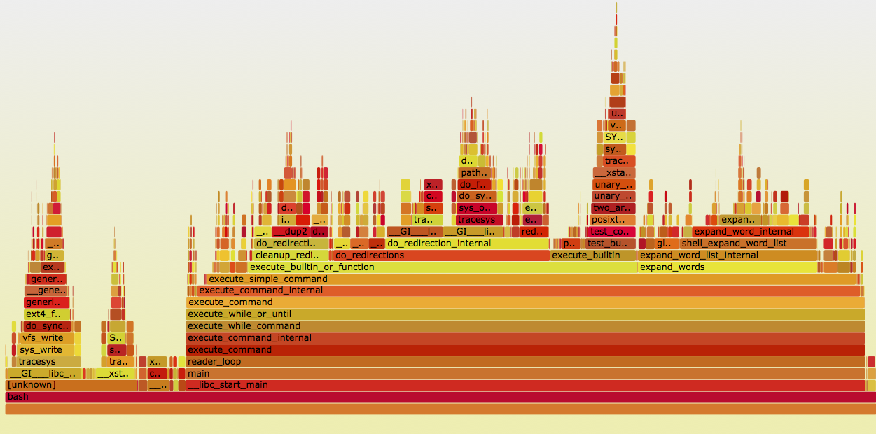
See http://www.brendangregg.com/flamegraphs.html for details on how to produce such graphs for compiled code. Julia’s ProfileView.jl can build these automatically for Julia code, and the profvis package can produce an interactive web page for R profiles. (See the example here.)
Other profiling tools are Callgrind and gperftools.
Line profiling #
Some profiling tools can measure individual lines instead of whole function calls. This can be useful if your code isn’t cleanly split into many small functions. (But it should be!)
Line profiling isn’t as commonly used as function profiling; look at the profvis package for an R implementation.
Always measure your changes! #
It is too easy to do optimization voodoo: tweak one line, then another, then another, without knowing what is working and what is not.
Use your profiler to test if the optimizations are worthwhile. (Most optimizations add a complexity cost to your code.)
Remember that program execution time is a random variable with noise: you need more than one run to tell if a change mattered. Profile your code like a statistician!
Many languages provide microbenchmarking packages to do this for you. For example, in Python:
>>> import timeit
>>> timeit.timeit('"-".join(str(n) for n in range(100))', number=10000)
0.8187260627746582
>>> timeit.timeit('"-".join([str(n) for n in range(100)])', number=10000)
0.7288308143615723
>>> timeit.timeit('"-".join(map(str, range(100)))', number=10000)
0.5858950614929199
R has the microbenchmark package to do the same thing.
Activity #
R #
Update your copy of the documents repository (with git pull) and open the file
documents/Activities/profiling/example.R and the accompanying hw4-poisson.R.
Don’t run the code yet. Instead,
- Look through the code and try to understand how it works.
- Make a guess about which function or part might be the slowest.
Testing the ideas #
Now let’s profile it.
In example.R there are a few lines of code to run R’s statistical profiler.
Run it and look at the output with your group. (You may need to install a few
packages so the code can run.)
Python #
In the game Connect Four, players take turns dropping a token of their own color into a vertical grid with the goal of being the first to get four-in-a-row, either horizontally, vertically, or diagonally.
With numpy and scipy, use 2d-convolution to find positions on the
board that represent a winning move. Here, the board is an
an m by n array with three distinct values corresponding to
empty, first player’s, and second player’s tokens.
Memory profiling #
Memory allocation has a cost. In my research, I had to fit a large mixture model, which required two ~10000x1000 (80 MB) mixing matrices on every iteration. As the data size grew, Python eventually ran out of memory on my 1GB server account, despite the matrices technically fitting in RAM.
Why is allocation a problem?
Garbage collection #
R, Python, Julia, Ruby, Java, JavaScript, and all other dynamic languages are garbage collected (GCed): at runtime, the interpreter must determine which variables are accessible (live) and which are not (garbage) and free memory accordingly.
In C and some other compiled languages, memory management is manual. There is a distinction between the stack and the heap:
- Stack
- When a function is called, its arguments are pushed onto the stack, as well as any local variables it declares, in a stack frame. When the function returns, its frame is popped off the stack, destroying the local variables. But the stack frame has a fixed size, and can only contain variables whose sizes are known in advance.
- Heap
- A global pool of explicitly-allocated memory. Can contain arbitrary objects shared between functions, but requires explicit management to allocate and deallocate space.
double fit_big_model(double *data, int p, double tuning_param, ...) {
  double *betas = malloc(p * sizeof(double));

  // do stuff

  free(betas);
}
More advanced languages like C++, Rust, D and so on add additional ways to manage memory, like RAII, which make it less cumbersome and less error-prone. (Rust uses ownership types to control memory use without GC.)
In dynamic languages, any object can be any size, and may live arbitrarily long. A typical strategy is tracing: the language keeps track of reachable objects, those referenced by local variables or global variables. It then traces out a graph: any object contained inside a local variable (e.g. inside a list in R) or accessible from one.
This produces the set of “live” objects. Any other objects are garbage and can be deallocated, since they are no longer accessible.
(This is essentially a graph traversal problem, and so there are many variations with different performance characteristics in different use cases.)
This traversal takes time. Most garbage collectors “stop the world”: execution stops while they collect. If there’s lots of garbage or lots of allocation, GC can be slow.
Tracking memory use #
Some languages provide simple blunt instruments to see how much memory is allocated by code:
julia> @time f(10^6)
elapsed time: 0.04123202 seconds (32002136 bytes allocated)
2.5000025e11
Memory profiling (sometimes called “heap profiling”) is not as common as ordinary profiling, but can still be very useful. There are a number of tools for different languages. Python’s memory_profiler module offers line-by-line memory profiling features. A simple example from its documentation:
@profile
def my_func():
    a = [1] * (10 ** 6)
    b = [2] * (2 * 10 ** 7)
    del b
    return a

if __name__ == '__main__':
    my_func()
Line #    Mem usage  Increment   Line Contents
==============================================
     3                           @profile
     4      5.97 MB    0.00 MB   def my_func():
     5     13.61 MB    7.64 MB       a = [1] * (10 ** 6)
     6    166.20 MB  152.59 MB       b = [2] * (2 * 10 ** 7)
     7     13.61 MB -152.59 MB       del b
     8     13.61 MB    0.00 MB       return a
These results are not wholly reliable, since they rely on the OS to report memory usage instead of tracking specific allocations, and garbage collection can occur unpredictably.
R’s Rprof has memory profiling, and its output is shown in provis when you
use the profiler in RStudio.
The valgrind tools suite (including in particular memcheck) provides powerful
tools for memory profiling (and other things) in programs compiled
with the C-toolchain.
Reducing allocations #
Common memory pitfalls include unnecessary copying:
foo <- function(x) {
    x$weights <- calculate_weights(x)

    s <- sample_by_weight(x)

    ...
}
Because we’ve written to x, x is copied. (This is peculiar to R’s
copy-on-write scheme.) Another example:
for (x in data) {
    results <- c(results, calculate_stuff(x))
}
The same happens with repeated rbind or cbind calls. Allocate results in
advance, or use Map or vapply instead:
results <- numeric(nrow(data))

for (i in seq_along(data)) {
    results[i] <- calculate_stuff(data[i])
}

## or:

results <- Map(calculate_stuff, data)

# (depending on if data is a list, vector, data frame...)
Intermediate results also require allocations:
pois.grad <- function(y, X) {
    function(beta) {
        t(X) %*% (exp(X %*% beta) - y)
    }
}
In Numpy, we can specify the output array to avoid these kinds of problems, with extra tedium:
def pois_grad(y, X):
    def grad(beta):
        tmp = np.empty((X.shape[0], 1))
        np.dot(X, beta, out=tmp)
        np.exp(tmp, out=tmp)
        np.subtract(tmp, y, out=tmp)

        return X.T * tmp

    return grad
I do not recommend writing code this ugly unless absolutely necessary. Numba is a smart optimizing compiler for Python code which can perform these kinds of optimizations automatically.
Resources #
- Python’s profiling documentation
- RStudio’s profiling documentation
- Rprof documentation
- Advanced R’s Profiling chapter
- RStudio’s profvis package for interactive profiling
- gprof
- Valgrind for a variety of memory and profiling tools for compiled code (typically C and C++)
General performance tips #
- The Cython optimizing compiler for Python
- Rcpp for R and C++ integration
- The R Inferno: “If you are using R and you think you’re in hell, this is a map for you.”
- Why Python is Slow, a blog post on the complicated abstractions buried inside Python that make it slow. Applies in part to other dynamic languages like R.
- A debugging and profiling story.