Today, we consider an algorithmic strategy, called dynamic programming, for a broad class of combinatorial optimization problems. The central ideas are that we
- decompose a problem into sub-problems,
- the sub-problems are organized into a DAG, and
- we remember the solutions to sub-problems we have already solved.
The term “programming” here is used in the old sense: referring to planning, scheduling, routing, assignment – and the optimization thereof. As with “linear programming,” “quadratic programming,” and “mathematical programming” you can think of it as a synonym for optimization. (The name was chosen by Richard Bellman in the 1950s essentially because it sounded cool and interesting, and hence the Air Force, which was funding his research, wouldn’t notice that he was actually just doing mathematics research.)
Illustrative Examples #
Fibonacci Revisited #
We saw earlier a simple recursive algorithm for computing Fibonacci numbers.
fib(n):
   if n == 0: return 0
   if n == 1: return 1
   return fib(n-1) + fib(n-2)
Recall that this does not perform well. Why?
fib(7) -> fib(6) -> fib(5), fib(4) -> fib(4), fib(3), fib(3), ...
          fib(5) -> fib(4), fib(3)
Because we end up recomputing the same value multiple times.
Two key strategies:
- Solve the problem in a particular order (from smaller
nto largern). - Store the solutions of problems we have already solved (memoization).
Together these strategies give us a performant algorithm.
Compare:
type Phi = Phi Integer Integer

instance Monoid Phi where
  munit = Phi 1 0
  mdot (Phi a b) (Phi m n) = Phi (a*m + b*n) (a*n + b*(m + n))

fib n = extract (fastMonoidPow n (Phi 0 1))
  where extract (Phi _ b) = b
Shortest Distance #
Consider a (one-way) road network connecting sites in a town, where each path from a site to a connected site has a cost.
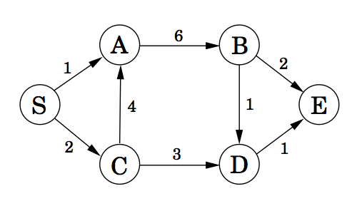
What is the lowest-cost path from S to E? How do we find it?
Solution #
Start from E and work backward.
- The best route from E to E costs 0.
- The best route from D to E costs 1.
- The best route from B to E costs 2.
- The best route from A to E costs 8.
- The best route from C to E costs 4.
- The best route from S to E costs 6. [S -> C -> D -> E]
Why does this work? #
The lowest-cost path from a given node to E is a subproblem of the original.
We can arrange these subproblems in an ordering so that we can solve the easiest subproblems first and then solve the harder subproblems in terms of the easier ones.
What ordering?
This is just a topological sort of the DAG that we saw
above. This gives us the subproblems in decreasing order:
S, C, A, B, D, E, though in practice we often handle
the subproblems in increasing order.
Overview: Dynamic Programming (DP) #
-
Decompose a problem into (possibly many) smaller subproblems.
-
Arrange those subproblems in the order they will be needed.
-
Compute solutions to the subproblems in order, storing the solution to each subproblem for later use.
-
The solution to a subproblem combines the solutions to earlier subproblems in a specific way.
Reminder: Topological Sorting DAGS #
A topological sort of a DAG is a linear ordering of the DAG’s nodes such that if \((u,v)\) is a directed edge in the graph, node \(u\) comes before node \(v\) in the ordering.
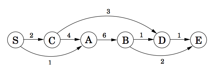
Example: A directed graph
and a rearrangment showing a topological sort
The sorted nodes are S C A B D E, which is decreasing order. For a general DAG, how do we use DFS to do a topological sort?
The Key Ideas Revisited #
-
Decompose a problem into smaller subproblems.
Implicitly, each subproblem is a node in a directed graph, and there is a directed edge \((u,v)\) in that graph when the result of one subproblem is required in order to solve the other.
\((v,u)\) is an edge when the result of solving subproblem \(v\) requires the result of subproblem \(u\).
-
Arrange those subproblems in the topologically sorted order of the graph.
A topological sort of the underlying DAG yields an ordering of the subproblems. We will call the subproblem order decreasing if it follows the directions of edges in the above graph; increasing if it goes against the edges.
-
Compute solutions to the subproblems in order, storing the result of each subproblem for later use if needed. This storing approach is called memoization or caching.
One common scenario is when you have a function to calculate the solution to a single subproblem, and we store our previous solution by memoizing the function. That is, when we call the function, we check if we have called it with these particular arguments before. If so, return the previously computed value. Otherwise, compute the value and store it, marking these arguments as being previously computed.
-
The solution to a subproblem combines the solutions to earlier subproblems through a specific mathematical relation.
The mathematical relationship between a subproblem solution and the solution of previous subproblems is often embodied in an equation, or set of equations, called the Bellman equations. We will see examples below.
Question #
For the Fibonacci example we just saw, what are the subproblems? What is the DAG? What does memoizing look like?
Exercise: Memoizing #
Write a function that memoizes its arguments.
Preliminary Example: Shortest Path in a Graph #
Above, we saw Dijkstra’s single-source shortest path algorithm; I claim that this is a dynamic programming problem.
We considered a (one-way) road network connecting sites in a town, where each path from a site to a connected site has a cost.
What is the lowest-cost path from S to E? How did we find it?
Formalizing our Solution #
For nodes \(u\) in our graph, let \(\mathrm{dist}(u)\) be the minimal cost of a path from \(u\) to \(E\) (the end node). We want \(\mathrm{dist}(S)\). Finding \(\mathrm{dist}(u)\) is a subproblem.
For subproblem nodes \(u, v\) with an edge \(u \to v\) connecting them, let \(c(u,v) \equiv c(v,u)\) be the cost of that edge.
Here is our algorithm:
-
Initialize \(\mathrm{dist}(u) = \infty\) for all \(u\).
-
Set \(\mathrm{dist}(E) = 0\).
-
Topologically sort the graph, giving us a sequence of nodes from S to E. Call this “subproblem dependent order”.
-
Work through the sorted nodes in reverse. For each node \(v\), set
\[ \mathrm{dist}(v) = \min_{u \to v} \left(\mathrm{dist}(u) + c(u,v)\right) \]
These last equations are called the Bellman equations.
Let’s try it. The subproblem dependent order is S, C, A, B, D, E, yielding:
dist(E) =                                 0
dist(D) = dist(E) + 1                   = 1
dist(B) = min(dist(E) + 2, dist(D) + 1) = 2
dist(A) = dist(B) + 6                   = 8
dist(C) = min(dist(A) + 4, dist(D) + 3) = 4
dist(S) = min(dist(A) + 1, dist(C) + 2) = 6
Exercise #
Write a function min_cost_path that returns the minimal cost
path to a target node from every other node in a weighted,
directed graph, along with the minimal cost. If there is no
directed path from a node to the target node, the path
should be empty and the cost should be infinite.
Your function should take a representation of the graph and a list of nodes in subproblem order. You can represent the graph anyway you prefer; however, one convenient interface, especially for R users, would be:
min_cost_path(target_node, dag_nodes, costs)
where target_node names the target node, dag_nodes lists all the nodes in
increasing order, and costs is a symmetric matrix of edge weights with rows
and columns arranged in dependent order. Assume: costs[u,v] = Infinity if
there is no edge between u and v.
Note: You can use the above example as a test case.
Example #2: Edit Distance #
When you make a spelling mistake, you have usually produced a “word” that is close in some sense to your target word. What does close mean here?
The edit distance between two strings is the minimum number of edits – insertions, deletions, and character substitutions – that converts one string into another.
Example: Snowy vs. Sunny. What is the edit distance?
Snowy
Snnwy
Snny
Sunny
Three changes transformed one into the other.
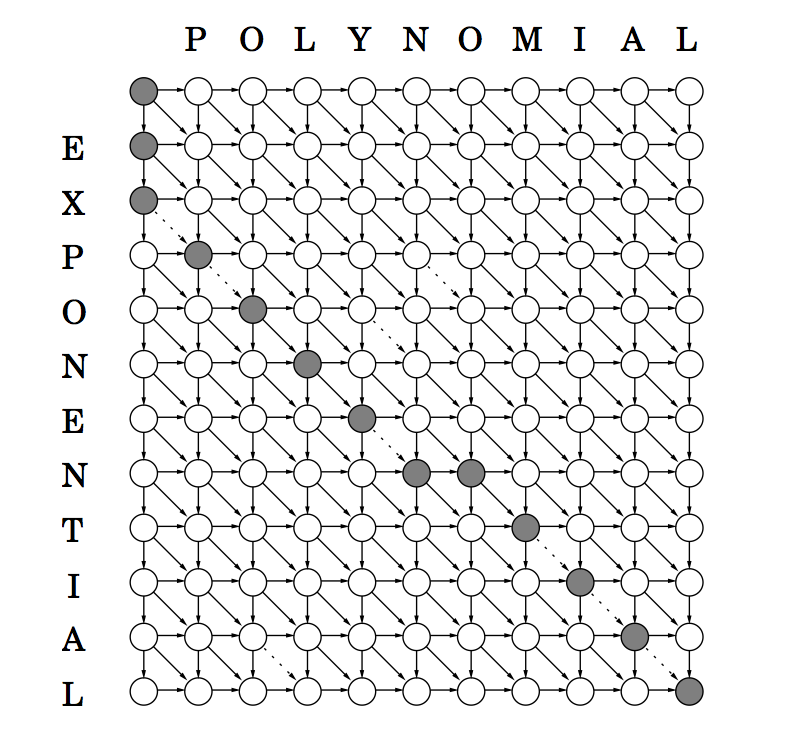
An equivalent but easier way to look at this is to think of it as
an alignment problem. We use a _ marker to indicate inserts
and deletions. Here are two possible alignments of Snowy and Sunny:
S _ n o w y                         _ S n o w _ y
S u n n _ y                         S u n _ _ n y

0 1 0 1 1 0   Total cost: 3         1 1 0 1 1 1 0   Total cost: 5
We can convince ourselves that the minimum cost here is 3,
and that is the edit distance edit(Snowy, Sunny).
But there are many possible alignments of two strings, and searching for the best among them would be costly.
Instead, we think about how to decompose this problem into sub-problems.
Consider computing edit(s, t) for two strings s[1..m], and t[1..n].
The sub-problems should be smaller versios of the same problem
that help us solve the bigger versions.
We can look at prefixes of the strings s[1..i] and t[1..j] as
the sub-problems, and express its solutions in terms of smaller
problems of the same form. Let E_ij = edit(s[1..i], t[1..j]).
When we find the best alignment of these strings, the last column in the table will be one of three forms
s[i]     _      s[i]
 _      t[j]    t[j]
The first case gives cost 1 + edit(s[1..i-1], t[1..j]).
The second case gives 1 + edit(s[1..i], t[1..j-1]).
The third case gives (s[i] != t[j]) + edit(s[1..i-1], t[1..j-1]).
Hence,
\[
E_{ij} = \min(1 + E_{i-1,j}, 1 + E_{i,j-1}, d_{ij} + E_{i-1,j-1}).
\]
We also have the initial conditions \(E_{i0} = i\) and \(E_{0j} = j\).
Hence, we can make a two dimensional table of sub-problems, which we can tackle in any order as long as \(E_{ij}\) is computed after \(E_{i-1,j}, E_{i, j-1}, E_{i-1,j-1}\).
What is the DAG here? If we weight the edges, we can get generalized costs.
Exercise: Finding the transform #
Write a function to compute the edit distance between two strings and a sequence of transformations of one string into the other.
What information do you need to keep track of? How do you organize the data? What types do you need?
Apply this to EXPONENTIAL and POLYNOMIAL
Example #3: Matrix Multiplication Order #
Suppose we have three matrices \(A\), \(B\), and \(C\). To compute \(ABC\), we have two choices \((AB)C\) or \(A(BC)\). Which is better?
Assuming standard matrix multiplication, multiplying an \(n\times p\) by a \(p \times r\) takes \(O(npr)\) operations.
Example: Suppose \(A\), \(B\), and \(C\) are respectively \(100 \times 20\), \(20 \times 100\) and \(100 \times 20\).
- \((AB)C\) takes \(100\cdot 20 \cdot 100 + 100 \cdot 100 \cdot 20 = 2\cdot 20\cdot 100^2\)
- \(A(BC)\) takes \(100\cdot 20 \cdot 20 + 20\cdot100\cdot 20 = 2\cdot 20^2 \cdot 100\)
This is a factor of 5 difference.
Problem*: Given matrices \(A_1, \ldots, A_n\) and their dimensions, what is the best way to “parenthesize” them in computing the products?
There are exponentially many choices, so brute force is out.
One might think that a greedy solution would work well, where we choose the cheapest pair at any point. But that doesn’t work.
For example: \(A 50\times 20\), \(B 20 \times 1\), \(C 1 \times 10\), and \(D 10\times 100\).
| A((BC)D) | 120,200 |
|---|---|
| (A(BC))D | 60,200 |
| (AB)(CD) | 7,000 |
The second choice is greedy.
Subproblems: We can think of each choice of parenthesization as giving a binary tree. For a particular tree to be optimal, its subtrees must also be optimal.For each pair \(i \le j\), parenthesize \(A_i \cdots A_j\), which has \(|j - i|\) matrix multiplications.
When \(i = j\), we have cost \(M(i,i) = 0\). If we look at cost \(M(i,j)\), we can consider all trees \(A_1\dotsb A_k\) and \(A_{k+1}\dotsb A_j\) for \(i \le k < j\). \[ M(i,j) = \min_{i \le k < j} \left[M_{ik} + M_{k+1,j} + r_i c_k c_j\right], \] where \(A_i\) is \(r_i \times c_i\) and \(c_i = r_{i+1}\).
This gives \(n^2\) subproblems. This is \(O(n)\) for each subproblem, giving \(O(n^3)\) total. (We can improve this.)
More Examples and Applications #
Example #4: Knapsack Problem #
We have \(n\) items to pick from with weights \(w_1, \dotsc, w_n\) and values \(v_1, \dotsc, v_n\). We have a knapsack that can accept a maximum weight of \(W\).
If we can take as many copies of each item as we like, what is the optimal value of what we can carry in a knapsack? What are the sub-problems? What is the DAG?
If we don’t allow repetitions, the subproblems and Belleman equations change
Example #5: Longest Increasing Subsequence #
Given a sequence s of n ordinals, find the longest
subsequence whose elements are strictly increasing.
5, 2, 8, 6, 3, 6, 9, 7 -> 2, 3, 6, 9
Let’s sketch a dynamic-programming solution for this problem. Work with a partner to answer these questions.
- What are the subproblems?
- Are they arranged in a DAG? If so, what are the relations?
- What are the Bellman equations for these subproblems?
- Sketch the DP algorithm here.
- We can find the longest length, how do we get the path?
- How would a straightforward recursion implementation perform? What goes wrong?
Example #5: Hidden Markov Models and Reinforcement Learning #
Hidden Markov Models #
In a Hidden Markov Model, the states of a system follow a discrete-time Markov chain with initial distribution \(\alpha\) and transition probability matrix \(P\), but we do not get to observe those states.
Instead we observe signals/symbols that represent noisy measurements of the state. In state \(s\), we observe symbol \(y\) with probability \(Q_{sy}\). These measurements are assumed conditionally independent of everything else given the state.
This model is denoted HMM\(\langle\alpha,P,Q\rangle\).
Many applications:
- Natural language processing
- Bioinformatics
- Image Analysis
- Learning Sciences
- …
If we denote the hidden Markov chain by \(X\) and the observed signals/symbols by \(Y\), then there are fast recursive algorithms for finding the marginal distribution of a state given the observed signals/symbols and the parameters.
But usually, we want to reconstruct the sequence of hidden states. That is, we want to find:
\[ \mathop{\rm argmax}\limits_{s_{0..n}} P_\theta\left\{ X_{0..n} = s_{0..n} \mid Y_{0..n} = y_{0..n} \right\} \]
It is sufficient for our purposes to solve a related problem
\[ v_k(s) = \mathop{\rm argmax}\limits_{s_{0..k-1}} P_\theta\left\{ X_{0..k-1} = s_{0..k-1}, X_k = s, Y_{0..k} = y_{0..k} \right\} \]
Then we have
\[ v_k(s) = Q_{s,y_k} \max_r P_{rs} v_{k-1}( r), \]
which gives us a dynamic programming solution.
\[ \max_s v_n(s) = Q_{w_n,y_n} \max_r P_{r,w_n} v_{n-1} ( r) \]
where \(w_n = {\rm argmax}_s v_k(s)\).
This is a DAG of subproblems.
Reinforcement Learning #
Reinforcement Learning builds on a similar representation where we have a Markov chain whose state transitions we can influence through actions. We get rewards and penalties over time depending on what state the chain is in.
We learn by interacting with our environment: making decisions, taking actions, and then (possibly much later) achieving some reward or penalty.
Reinforcement learning is a statistical framework for capturing this process.
A goal-directed learner, or agent, learns how to map situations (i.e., states) to actions so as to maximize some numerical reward.
- The agent must discover the value of an action by trying it.
- The agent’s actions may affect not only the immediate reward but also the next state – and through that the downstream rewards as well.
These two features – value discovery and delayed reward – are important features of the reinforcement learning problem.
-
Examples
-
Playing tic-tac-toe against an imperfect player.
-
The agent plays a game of chess against an opponent.
-
An adaptive controller adjusts a petroleum refinery’s operation in real time to optimize some trade-off among yield, cost, and quantity.
-
A gazelle calf struggles to stand after birth and is running in less than an hour.
-
An autonomous, cleaning robot searches for trash among several rooms but must take care to return to a recharging station when power gets low.
-
Phil prepares his breakfast.
Common themes: interaction, goals, rewards, uncertainty, planning, monitoring
-
-
Elements of Reinforcement Learning
-
The agent – the entity that is learning
-
The environment – the context in which the agent is operating, often represented by a state space.
-
A policy – determines the agent’s behavior.
It is a function mapping from states of the environment to actions (or distributions over actions) to take in that state.
-
A reward function – defines the agent’s goal.
It maps each state or each state and action pair to a single number (called the reward) that measures the desirability of that state or state-and-action.
The reward at any state (or state-action pair) is immediate. The agent’s overall goal is to maximize the accumulated reward.
-
A value function – indicates the accumulated desirability of each state (or state-action pair).
Roughly speaking, the value function at a state is the expected accumulated reward an agent can receive starting at that state (by choosing ``good’’ actions). The value function captures the delayed rewards.
-
An environment model (Optional) – mimics the environment for planning purposes.
-
-
Markov Decision Processes
We model reinforcment using a Markov Decision Process.
This is a discrete-time stochastic process on a state space S where the probabilities of transitions between states are governed by Markov transition probabilities for each action the agent can choose from a set A.
The goal is to maximize the cumulative reward (possibly discounted) over time (with reward r(X_k) at time k).
Using the Markov structure of the process allows us to find good (or even optimal) decision policies.
Application: Fast file differences #
Programs diff, git-diff, rsync use such algorithms (along with related dynamic programming problem Longest Common Subsequence) to quickly find meaningful ways to describe differences between arbitrary text files.
Application: Genetic Alignment #
Use edit distance logic to find the best alignment between two sequences of genetic bases (A, T, C, G). We allow our alignment to include gaps (’_’) in either or both sequences.
Given two sequences, we can score our alignment by summing a score at each position based on whether the bases match, mismatch, or include a gap.
C G A A T G C C A A A
C A G T A A G G C C T T A A

C _ G _ A A T G C C _ A A A
C A G T A A G G C C T T A A
m g m g m m x m m m g x m m

Score = 3*gap + 2*mismatch + 9*match
With (sub-)sequences, S and T, let S’ and T’ respectively, be the sequences without the last base. There are then three subproblems to solve to align(S,T):
- align(S,T')
- align(S’,T)
- align(S’,T')
The score for S and T is the biggest score of:
- score(align(S,T’)) + gap
- score(align(S’,T)) + gap
- score(align(S’,T’)) + match if last characters of S,T match
- score(align(S’,T’)) + mismatch if last characters do not match
The boundary cases (e.g., zero or one character sequences) are easy to compute directly.
Question: Longest Common Subsequence #
If we want to find the longest common subsequence (LCS) between two strings, how can we adapt the logic underlying the edit distance example to find a dynamic programming solution?