A graph is a structure that represents the relationships among a set of entities. It consists of
- A set of nodes (also called vertices) representing the entities.
- A set of edges each connecting two nodes.
Two nodes connected by an edge are called neighbors, or adjacent.
Graphs are enormously important in statistics, in computing, and more generally. Many things can be treated as graphs:
- Social networks, where nodes are people and edges are relationships between them
- Statistical models, where nodes are variables and edges represent dependence, causality, or correlation
- Road maps, where nodes are intersections and buildings and edges represent connections between them via road
- Electric circuits, where nodes are circuit nodes and edges the resistors, inductors, and capacitors connecting them
- The Internet is a bunch of nodes (routers and individual computers) connected by Ethernet, WiFi, ISPs, undersea cables…
Treating something complicated, like a social network, as a graph lets us apply a range of powerful tools to work with it. By learning generally about graphs, we learn tools that can be used for many different kinds of problems.
Rather than remembering the details of various graph algorithms, it is useful to think about common graph problems and how they apply to your situation. Finding good algorithms then follows fairly easily.
Common graph problems:
- Finding connected components
- Finding shortest paths
- Matching and coloring
- Transitive closure
- Finding a minimal spanning tree
- Traversing the graph
- Topological sorting
- Finding separating edges and nodes
- Finding cycles and “tours”
- Maximizing flows through a network
- Calculating useful embeddings.
But first, let’s learn about graphs.
Flavors of Graphs #
Mathematically, a graph \(G = (N, E)\), where \(N\) is a set of nodes and \(E\) is a set containing 2-sets of the form \(\{n_1, n_2\}\), that represents an edge between nodes \(n_1\) and \(n_2\). (They are 2-sets because they are not ordered: \(\{n_2, n_1\}\) represents the same edge as \(\{n_1, n_2\}\).)
A graph is connected if one can move between any two nodes by a series of steps between adjacent nodes. That is, any node is a neighbor of a neighbor of a neighbor of a… of any other node.
Graphs are often shown, er, graphically with the nodes as circles (or other shapes) and the edges as lines or curves linking the nodes.
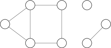
A graph can be basic, like a single node with no edges, or complex, like:
Properties (especially Labels and Weights) #
While the nodes and edges define the relationships, we often want to encode more information. To that end, we can associate properties with the nodes and the edges. These properties can be arbitrary data (or meta-data), but most common are labels and weights, which are strings and numbers, respectively, associated with nodes and/or edges.
Here is a graph with labeled nodes:
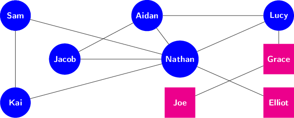
Here is a graph with labeled nodes and weighted edges:

Weights might be used to represent many things: the strength of correlation between variables, the distance between two points on the road network, or the number of emails sent between two people, among many other potential applications.
Directed versus Undirected Graphs #
The graphs displayed above are undirected: the edges \(\{n_1, n_2\}\) represent symmetric relationships between the nodes. For example, Kai is friends with Nathan if and only if Nathan is friends with Kai.
In contrast, a directed graph, or digraph, has edges with direction that represent asymmetric relationships. For example, Joe might “like” Grace without Grace liking Joe.
Mathematically, the edges in a digraph are not sets but tuples, specifically ordered pairs \((n_1, n_2)\) representing an edge from node \(n_1\) to node \(n_2\).
Graphically, we display directed edges as arrows:

Simple versus Non-Simple #
A simple graph has
- no edges from a node to itself,
- at most one edge between any pair of nodes;
otherwise, the graph is non-simple. The graphs above were all simple; here’s a non-simple example.
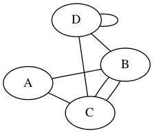
Most graphs we work with are simple graphs.
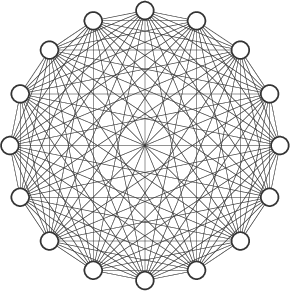
Sparse versus Dense #
A graph is sparse if only a small fraction of the possible edges are present; otherwise it is dense. Which of the examples above are sparse? Which are dense?
Later we’ll see that the difference between a sparse and a dense graph has implications for how we choose to represent a graph in our programs.
Consider a large social network, like Facebook, where edges represent “friendship” between two members. Is such a graph sparse or dense?
Cyclic versus Acyclic #
A cycle in a digraph is a sequence of adjacent nodes (a path, respecting direction) that begin and end with the same node. (There are several different flavors of cycle.)
An acyclic graph has no cycles (else it is cyclic). A directed, acyclic graph is called a DAG.
One of the most important types of acyclic graph is a tree.
A graph G is a tree if any of the following (equivalent) properties hold:
- G is connected, acyclic graph.
- G is connected but deleting any edge makes it disconnected.
- Any two distinct nodes in G are connected by exactly one simple path (a path containing distinct nodes only).
- A finite G with \(n\) nodes is a tree if it is acyclic and has \(n - 1\) edges.
- A finite G with \(n\) nodes is a tree if it is connected and has \(n - 1\) edges.
There are many varieties of tree. Here’s a binary tree, for example, where each node has only two children:

Representing Graphs #
There are several common data structures used to represent graphs. For a graph \(G\), let \(n = \#N\) and \(e = \#E\) denote the total number of nodes and edges.
When we talked about data structures, we made a distinction between the abstract operations a data structure supports and the actual implementation, in code and in memory, of the data structure. The same applies here: a graph is an abstract idea, and there are a few operations we want it to support:
- Check if there is an edge between two nodes
- Add and remove nodes
- Add and remove edges between nodes
- List the neighbors of a node
- Traverse the graph
Let’s discuss a few common implementations, which have different tradeoffs in computational complexity and storage costs.
Adjacency Matrix #
An \(n \times n\) matrix where an entry at row \(i\) and column \(j\) indicates whether there is an edge connecting \(i\) and \(j\). In digraphs, rows represent source nodes and columns represent destination nodes. In undirected graphs, adjacency matrices are symmetric.
Adjacency matrices make it easy to look up whether an edge exists. They are useful for dense, simple graphs. Properties must be stored elsewhere.
| A | B | C | D | E | F | G | |
|---|---|---|---|---|---|---|---|
| A | 0 | 1 | 1 | 0 | 0 | 0 | 0 |
| B | 1 | 0 | 0 | 1 | 1 | 0 | 0 |
| C | 1 | 0 | 0 | 0 | 0 | 1 | 1 |
| D | 0 | 1 | 0 | 0 | 0 | 0 | 0 |
| E | 0 | 1 | 0 | 0 | 0 | 0 | 0 |
| F | 0 | 0 | 1 | 0 | 0 | 0 | 0 |
| G | 0 | 0 | 1 | 0 | 0 | 0 | 0 |
In graphs with weighted edges, the adjacency matrix often stores the weights on each edge instead of 1. Instead of 0 for no-edge, it is sometimes convenient to use \(\infty\).
Adjacency List #
For each node, we store a list of the node’s neighbors:
| Node | Neighbors |
|---|---|
| A | B |
| B | A C U |
| C | B U E F G |
| U | B C |
| E | C F |
| F | C E G |
| G | C F |
We can allow self links and multi-links (via repeats in the list). We can also store data (or a pointer to it) in the list.
Incidence Matrix #
An \(n \times e\) boolean matrix, where rows represent nodes and columns represent edges, and where the \(i,j\) element being true means that node \(i\) is “incident on” edge \(j\).
Operations and Performance #
| Operation | Adjacency Matrix | Adjacency List | Incidence Matrix | Winner |
|---|---|---|---|---|
| u, v adjacent? | O(1) | O(n) | O(e) | Adjacency Matrix |
| degree(u) | O(n) | O(neighbors) | O(e) | Adjacency List |
| insert node | O(n^2) | O(1) | O(n e) | Adjacency List |
| insert edge | O(1) | O(neighbors) | O(n e) | Adjacency List |
| delete node | O(n^2) | O(e) | O(n e) | depends |
| delete edge | O(1) | O(e) | O(n e) | Adjacency Matrix |
| memory (small G) | O(n^2) | O(n + e) | O(n e) | Adjacency List |
| memory (big G) | O(n^2) | O(n + e) | O(n e) | Adjacency Matrix |
| traversal | Theta(n + e) | Theta(n^2) | Adjacency List |
Adjacency lists are a good default, but pay attention to the problem at hand.
Group Exercise #
Design two data structures/classes that represent an undirected graph in the Adjacency Matrix and List representation, respectively.
You can assume the nodes are identified by numbers from 1..n or 0..(n-1), whichever is more convenient.
For example, if you choose classes:
- What are the class names?
- What data do they contain?
- What methods should they have and what are their arguments?
- How do you ensure that adjacency matrix and adjacency list implementations are interchangeable with each other?
Ideas?