SQL

Introducing SQL and Postgres #

Getting Started #

Invoke psql at the shell prompt to start the PostgreSQL REPL.

Pull the documents repository to get access to the data files for today.

Getting Help #

Type \? at the prompt to get a list of meta-commands (these are psql, not SQL, commands).

A few of these are quite common:

• \q quit psql
• \h provides help on an SQL command or lists available commands
• \d list or describe tables, views, and sequences
• \l lists databases
• \c connect to a different database
• \i read input from a file (like source)
• \o send query output to a file or pipe
• \! execute a shell command
• \cd change directory

The PostgreSQL manual is a well-written and valuable resource.

Help for writing SQL queries, finding functions in Postgres, ….

Entering SQL Statements #

SQL consists of a sequence of statements.

Each statement is built around a specific command, with a variety of modifiers and optional clauses.

Keep in Mind:

• Command names and modifiers are not case-sensitive.

• SQL statements can span several lines, and all SQL statements end in a semi-colon (;).

• Strings are delimited by single quotes ’like this’, not double quotes “like this”.

• SQL comments are lines starting with --.

A Simple Example #

Try the following (or copy it from the notes or commands-1.sql).

create table products (
       product_id SERIAL PRIMARY KEY,
       name text,
       price numeric CHECK (price > 0),
       sale_price numeric CHECK (sale_price > 0),
       CHECK (price > sale_price)
);

Then type \d at the prompt. You should see the table.

Next, we will enter some data.

INSERT INTO products (name, price, sale_price) values ('furby', 100, 95);
insert into products (name, price, sale_price)
       values ('frozen lunchbox', 10, 8),
              ('uss enterprise', 12, 11),
              ('spock action figure', 8, 7),
              ('slime', 1, 0.50);

Do the following, one at a time.

select * from products;
select name, price from products;
select name as product, price as howmuch from products;

Discussion…

Making Tables #

Creating Tables #

We use the CREATE TABLE command. In its most basic form, it looks like

create table NAME (attribute1 type1, attribute2 type2, ...);

A simple version of the previous products table is:

create table products (
       product_id integer,
       name text,
       price real,
       sale_price real
);

This gets the idea, but a few wrinkles are nice. Here’s the fancy version again:

create table products (
       product_id SERIAL PRIMARY KEY,
       name text,
       price numeric CHECK (price > 0),
       sale_price numeric CHECK (sale_price > 0),
       CHECK (price > sale_price)
);

Discussion, including:

• Column product_id is automatically set when we add a row.
• We have told postgres that product_id is the primary key.
• Columns price and sale_price must satisfy some constraints.
• What happens if we try to add data that violates those constraints? Try this:

  insert into products (name, price, sale_price)
         values ('kirk action figure', 50, 52);
  

• There are two kinds of constraints here: constraints on columns and constraints on the table. Which are which?

Here’s an alternative approach to making the products table:

create table products (
       product_id SERIAL PRIMARY KEY,
       label text UNIQUE NOT NULL CHECK (char_length(label) > 0),
       price numeric CHECK (price >= 0),
       discount numeric DEFAULT 0.0 CHECK (discount >= 0),
       CHECK (price > discount)
);

Notice that there are a variety of functions that postgres offers for operating on the different data types. For instance, char_length() returns the length of a string.

Now, which one of these will work?

insert into products (label, price)
       values ('kirk action figure', 50);
insert into products (price, discount)
       values (50, 42);
insert into products (label, price, discount)
       values ('', 50, 42);

Altering Tables #

The ALTER TABLE command allows you to change a variety of table features. This includes adding and removing columns, renaming attributes, changing constraints or attribute types, and setting column defaults. See the full documentation for more.

A few examples using the most recent definition of products:

• Let’s rename product_id to just id for simplicity.

  alter table products
        rename product_id to id;
  

• Let’s add a brand_name column.

  alter table products add brand_name text DEFAULT 'generic' NOT NULL;
  

• Let’s drop the discount column

  alter table products drop discount;
  

• Let’s set a default value for brand_name.

  alter table products
        alter brand_name SET DEFAULT 'generic';
  

Deleting Tables #

The command is DROP TABLE.

drop table products;
drop table products cascade;

Try it, then type \d at the prompt.

This command is permanent and irreversible (unless you have a backup).

Working with CRUD #

The four most basic operations on our data are

• Create
• Read
• Update
• Delete

collectively known as CRUD operations.

In SQL, these correspond to the four core commands INSERT, SELECT, UPDATE, and DELETE.

To start our exploration, let’s create a table. Motivation: Suppose we have an online learning platform where students read course materials, watch videos, and take quizzes on the content. We’d like to record “events” every time a student takes a quiz.

create table events (
       id SERIAL PRIMARY KEY,
       moment timestamp DEFAULT 'now',
       persona integer NOT NULL,
       element integer NOT NULL,
       score integer NOT NULL DEFAULT 0 CHECK (score >= 0 and score <= 1000),
       hints integer NOT NULL DEFAULT 0 CHECK (hints >= 0),
       latency real,
       answer text,
       feedback text
);

Note: Later on, persona and element will be foreign keys, but for now, they will just be arbitrary integers.

INSERT #

The basic template is

INSERT INTO <tablename> (<column1>, ..., <columnk>)
       VALUES (<value1>, ..., <valuek>);

If the column names are excluded, then values for all columns must be provided. You can use DEFAULT in place of a value for a column with a default setting.

You can also insert multiple rows at once

INSERT INTO <tablename> (<column1>, ..., <columnk>)
       VALUES (<value11>, ..., <value1k>),
              (<value21>, ..., <value2k>),
              ...
              (<valuem1>, ..., <valuemk>);

You can add a RETURNING clause that makes the INSERT query return a table of results, which you can choose – such as the IDs of the inserted rows.

Examples #

First, copy data from events.csv into the events table: (modify the path to ’events.csv’ to be correct for your computer)

\COPY events FROM 'events.csv' WITH DELIMITER ',';
SELECT setval('events_id_seq', 1001, false);

If you’re connected to our SQL server, the path above will work, since the data is available in my home directory. Note that when you’re connected to our server, paths refer to locations on the server, not on your own computer.

insert into events (persona, element, score, answer, feedback)
       values (1211, 29353, 824, 'C', 'How do the mean and median differ?');
insert into events (persona, element, score, answer, feedback)
       values (1207, 29426, 1000, 'A', 'You got it!')
       RETURNING id;
insert into events (persona, element, score, answer, feedback)
       values (1117, 29433,  842, 'C', 'Try simplifying earlier.'),
              (1199, 29435,    0, 'B', 'Your answer was blank'),
              (1207, 29413, 1000, 'C', 'You got it!'),
              (1207, 29359,  200, 'A', 'A square cannot be negative')
       RETURNING *;

Try inserting a few valid rows giving latencies but not id or feedback. Find the value of the id’s so inserted.

SELECT #

The SELECT command is how we query the database. It is versatile and powerful command.

The simplest query is to look at all rows and columns of a table:

select * from events;

The * is a shorthand for “all columns.”

Selects can include expressions, not just column names, as the quantities selected. And we can use as clauses to name (or rename) the results.

select 1 as one;
select ceiling(10 * random()) as r;
select 1 as ones from generate_series(1,10);
select min(r), avg(r) as mean, max(r) from
       (select random() as r from generate_series(1, 10000)) as _;
select '2015-01-22 08:00:00'::timestamp + random() * '64 days'::interval
       as w from generate_series(1, 10);

Notice how we used a select to create a virtual table and then selected from it.

Most importantly, we can qualify our queries with conditions that refine the selection. We do this with the WHERE clause, which accepts a logical condition on any expression and selects only those rows that satisfy the condition. The conditional expression can include column names (even temporary ones) as variables.

select * from events where id > 20 and id < 40;

We can also order the output using the ORDER BY clause:

select score, element from events
    where persona = 1202
    order by element, score;

And we can limit the number of results using LIMIT:

select score, element from events
    where persona = 1202
    order by element, score
    limit 10;

Aggregate Functions and Grouping #

Aggregate functions operate on one or more attributes to produce a summary value. Examples: count, max, min, sum.

For example, let’s calculate the average score obtained by students:

select avg(score) from events;

This produces a single row: the average score. Any aggregate function takes many rows and reduces them to a single row. This is why you can’t write this:

select persona, avg(score) from events;

Try it; why does Postgres complain?

We often want to apply aggregate functions not just to whole columns but to groups of rows within columns. This is the province of the GROUP BY clause. It groups the data according to a specific value, and aggregate functions then produce a single result per group.

For example, if I wanted the average score for each separate user, I could write:

select persona, avg(score) as mean_score
from events
group by persona
order by mean_score desc;

You can apply conditions on grouped queries. Instead of WHERE for those conditions, you use HAVING, with otherwise the same syntax. Short version: WHERE select rows, and HAVING selects groups.

select persona, avg(score) as mean_score
from events
where moment > '2020-10-01 11:00:00'::timestamp
group by persona
having avg(score) > 50
order by mean_score desc;

Examples #

Try to craft selects in events for the following:

1. List all event ids for events taking place after 20 March 2015 at 8am. (Hint: > and < should work as you hope.)
2. List all ids, persona, score where a score > 900 occurred.
3. List all persona (sorted numerically) who score > 900. Can you eliminate duplicates here? (Hint: Consider SELECT DISTINCT)
4. Can you guess how to list all persona whose average score > 600. You will need to do a GROUP BY as above. (Hint: use HAVING instead of WHERE for the aggregate condition.)
5. Produce a table showing how many times each instructional element was practiced. The COUNT() aggregate function counts the number of rows in each group.

UPDATE #

The UPDATE command allows us to modify existing entries in any way we like. The basic syntax looks like this:

UPDATE table
    SET col1 = expression1,
        col2 = expression2,
        ...
    WHERE condition;

Beware: If you omit the WHERE clause, the update will be applied to every row.

The UPDATE command can update one or more columns and can have a RETURNING clause like INSERT.

Examples #

First we make a table of gems with some random data:

create table gems (label text DEFAULT '',
                   facets integer DEFAULT 0,
                   price money);

insert into gems
(select '', ceiling(20 * random() + 1), '1.00'::money
 from generate_series(1, 20) as k);

update gems set label = ('{thin,quality,wow}'::text[])[ceil(random() * 3)];

Now let’s do some updates:

update gems set label = 'thin'
       where facets < 10;
update gems set label = 'quality',
                price = 25.00 + cast(10 * random() as numeric)
       where facets >= 10 and facets < 20;
update gems set label = 'wow', price = '100.00'::money
       where facets >= 20;

select * from gems;

Now you try it (in the events table):

1. Set answer for id > 800 to the letter C.
2. Update the scores to subtract 50 points for every hint taken when id > 800. Check before and after to make sure it worked.

DELETE #

The DELETE command allows you to remove rows from a table that satisfy a condition. The basic syntax is:

DELETE FROM table WHERE condition;

Examples:

delete from gems where facets < 5;
delete from events where id > 1000 and answer = 'B';

Activity #

Here, we will do some brief practice with CRUD operations by generating a table of random data and playing with it.

1. Create a table rdata with five columns: one integer column id, two text columns a and b, one date moment, and one numeric column x. Be sure to list them in that order.

2. Fill the table with data using this command: (modify the path to ‘rdata.csv’ to be correct for your computer)

   \COPY rdata FROM 'rdata.csv' WITH DELIMITER ',';
   

   Use a SELECT to preview the first 10 rows so you see what kind of data is inside.

3. Use SELECT to display rows of the table for which b is equal to a particular choice.

4. Use SELECT with the overlaps operator on dates to find all rows with moment in the month of November 2017. You can find functions for working on dates and times in the manual if you need them.

   The OVERLAPS operator is a binary operator that can tell if two date intervals overlap:

   SELECT ('2020-10-01'::date, '2020-10-01'::date) OVERLAPS ('2020-09-24'::date, '2020-10-14'::date);
   

   Then use a query to calculate the minimum, maximum, and average of x for all rows whose moment is in the month of November.

5. Use UPDATE to set the value of b to a fixed choice for all rows whose id is divisible by 3 and 5.

6. Use DELETE to remove all rows for which id is even and greater than 2. (Hint: % is the mod operator.)

7. Use a few more DELETE’s (four more should do it) to remove all rows where id is not prime.

8. Use SELECT with either the ~* or ilike operators to display rows for which a matches a specific pattern, e.g.,

   select * from rdata where a ~* '[0-9][0-9][a-c]a';
   

Joins and Foreign Keys #

As we will see shortly, principles of good database design tell us that tables represent distinct entities with a single authoritative copy of relevant data. This is the DRY principle in action, in this case eliminating data redundancy.

An example of this in the events table are the persona and element columns, which point to information about students and components of the learning environment. We do not repeat the student’s information each time we refer to that student. Instead, we use a link to the student that points into a separate Personae table.

But if our databases are to stay DRY in this way, we need two things:

1. A way to define links between tables (and thus define relationships between the corresponding entities).

2. An efficient way to combine information across these links.

The former is supplied by foreign keys and the latter by the operations known as joins. We will tackle both in turn.

Foreign Keys #

A foreign key is a field (or collection of fields) in one table that uniquely specifies a row in another table. We specify foreign keys in Postgresql using the REFERENCES keyword when we define a column or table. A foreign key that references another table must be the value of a unique key in that table, though it is most common to reference a primary key.

Example:

create table countries (
       country_code char(2) PRIMARY KEY,
       country_name text UNIQUE
);
insert into countries
  values ('us', 'United States'), ('mx', 'Mexico'), ('au', 'Australia'),
         ('gb', 'Great Britain'), ('de', 'Germany'), ('ol', 'OompaLoompaland');
select * from countries;
delete from countries where country_code = 'ol';

create table cities (
       name text NOT NULL,
       postal_code varchar(9) CHECK (postal_code <> ''),
       country_code char(2) REFERENCES countries,
       PRIMARY KEY (country_code, postal_code)
);

Foreign keys can also be added (and altered) as table constraints that look like FOREIGN KEY (<key>) references <table>.

Now try this

insert into cities values ('Toronto', 'M4C185', 'ca'), ('Portland', '87200', 'us');

Notice that the insertion did not work – and the entire transaction was rolled back – because the implicit foreign key constraint was violated. There was no row with country code ‘ca’.

So let’s fix it. Try it!

insert into countries values ('ca', 'Canada');
insert into cities values ('Toronto', 'M4C185', 'ca'), ('Portland', '87200', 'us');
update cities set postal_code = '97205' where name = 'Portland';

Joins #

Suppose we want to display features of an event with the name and course of the student who generated it. If we’ve kept to DRY design and used a foreign key for the persona column, this seems inconvenient.

That is the purpose of a join. For instance, we can write:

select personae.lastname, personae.firstname, events.score, events.moment
       from events
       join personae on events.persona = personae.id
       where moment > '2015-03-26 08:00:00'::timestamp
       order by moment;

Joins incorporate additional tables into a select. This is done by appending to the from clause:

from <table> join <table> on <condition> ...

where the on condition specifies which rows of the different tables are included. And within the select, we can disambiguate columns by referring them to by <table>.<column>. Look at the example above with this in mind.

We will start by seeing what joins mean in a simple case.

create table A (id SERIAL PRIMARY KEY, name text);
insert into A (name)
       values ('Pirate'),
              ('Monkey'),
              ('Ninja'),
              ('Flying Spaghetti Monster');

create table B (id SERIAL PRIMARY KEY, name text);
insert into B (name)
       values ('Rutabaga'),
              ('Pirate'),
              ('Darth Vader'),
              ('Ninja');
select * from A;
select * from B;

Let’s look at several kinds of joins. (There are others, but this will get across the most common types.)

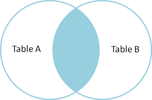
Inner Join #

An inner join produces the rows for which attributes in both tables match. (If you just say JOIN in SQL, you get an inner join; the word INNER is optional.)

select * from A INNER JOIN B on A.name = B.name;

We think of the selection done by the on condition as a set operation on the rows of the two tables. Specifically, an inner join is akin to an intersection:

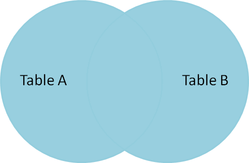
Full Outer Join #

A full outer join produces the full set of rows in all tables, matching where possible but null otherwise.

select * from A FULL OUTER JOIN B on A.name = B.name;

As a set operation, a full outer join is a union

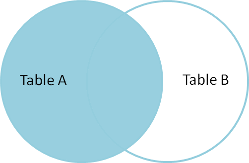
Left Outer Join #

A left outer join produces all the rows from A, the table on the “left” side of the join operator, along with matching rows from B if available, or null otherwise. (LEFT JOIN is a shorthand for LEFT OUTER JOIN in postgresql.)

select * from A LEFT OUTER JOIN B on A.name = B.name;

A left outer join is a hybrid set operation that looks like:

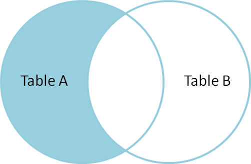
Set Difference #

Exercise: Give a selection that gives all the rows of A that are not in B.

select * from A LEFT OUTER JOIN B on A.name = B.name where B.id IS null;

This corresponds to a set difference operation A - B:

Symmetric Difference #

Exercise: Select the rows of A not in B and the rows of B not in A.

select * from A FULL OUTER JOIN B on A.name = B.name
    where B.id IS null OR A.id IS null;

This corresponds to a set difference operation A - B: ../Figures/left-outer-join-exclusions.png

A simple join exercise #

Using the cities and countries tables we created earlier, do the following:

1. List city name, postal code, and country name for each city.
2. List city name, country, and address as a valid string. (The concat() function takes multiple strings as arguments and concatenates them together.)

A bigger join exercise #

Now let’s create a venues table as well:

create table venues (
       id SERIAL PRIMARY KEY,
       name varchar(255),
       street_address text,
       type char(7) CHECK (type in ('public', 'private')) DEFAULT 'public',
       postal_code varchar(9),
       country_code char(2),
       FOREIGN KEY (country_code, postal_code)
         REFERENCES cities (country_code, postal_code) MATCH FULL
);
insert into venues (name, postal_code, country_code)
  values ('Crystal Ballroom', '97205', 'us'),
         ('Voodoo Donuts', '97205', 'us'),
         ('CN Tower', 'M4C185', 'ca');
update venues set type = 'private' where name = 'CN Tower';
select * from venues;

Now create a social_events with a few social events:

create table social_events (
       id SERIAL PRIMARY KEY,
       title text,
       starts timestamp DEFAULT 'now'::timestamp + '1 month'::interval,
       ends timestamp DEFAULT 'now'::timestamp + '1 month'::interval + '3 hours'::interval,
       venue_id integer REFERENCES venues (id)
);
insert into social_events (title, venue_id) values ('LARP Club', 3);
insert into social_events (title, starts, ends)
  values ('Fight Club', 'now'::timestamp + '12 hours'::interval,
          'now'::timestamp + '16 hours'::interval);
insert into social_events (title, venue_id)
  values ('Arbor Day Party', 1), ('Doughnut Dash', 2);
select * from social_events;

Exercise: List a) all social events with a venue with the venue names, and b) all social events with venue names even if missing.

When we know we will search on certain fields regularly, it can be helpful to create an index, which speeds up those particular searches.

create index social_events_title  on social_events using hash(title);
create index social_events_starts on social_events using btree(starts);

select * from social_events where title = 'Fight Club';
select * from social_events where starts >= '2015-11-28';

Database Schema Design Principles #

The key design principle for database schema is to keep the design DRY – that is, eliminate data redundancy. The process of making a design DRY is called normalization, and a DRY database is said to be in “normal form.”

The basic modeling process:

1. Identify and model the entities in your problem
2. Model the relationships between entities
3. Include relevant attributes
4. Normalize by the steps below

Example #

Consider a database to manage songs:

Album         Artist              Label     Songs
------------- ------------------- --------- ----------------------------------
Talking Book  Stevie Wonder       Motown    You are the sunshine of my life,
                                            Maybe your baby, Superstition, ...
Miles Smiles  Miles Davis Quintet Columbia  Orbits, Circle, ...
Speak No Evil Wayne Shorter       Blue Note Witch Hunt, Fee-Fi-Fo-Fum, ...
Headhunters   Herbie Hancock      Columbia  Chameleon, Watermelon Man, ...
Maiden Voyage Herbie Hancock      Blue Note Maiden Voyage
American Fool John Couger         Riva      Hurts so good, Jack & Diane, ...
...

This seems fine at first, but why might this format be problematic or inconvenient?

• Difficult to get songs from a long list in one column

• Same artist has multiple albums

• “Best Of” albums

• A few thoughts:

  • What happens if an artist changes names partway through his or her career (e.g., John Cougar)?
  • Suppose we want mis-spelled “Herbie Hancock” and wanted to update it. We would have to change every row corresponding to a Herbie Hancock album.
  • Suppose we want to search for albums with a particular song; we have to search specially within the list for each album.

The schema here can be represented as

Album (artist, name, record_label, song_list)

where Album is the entity and the labels in parens are its attributes.

To normalize this design, we will add new entities and define their attributes so each piece of data has a single authoritative copy.

Step 1. Give Each Entity a Unique Identifier #

This will be its primary key, and we will call it id here.

Key features of a primary key are that it is unique, non-null, and it never changes for the lifetime of the entity.

Step 2. Give Each Attribute a Single (Atomic) Value #

What does each attribute describe? What attributes are repeated in Albums, either implicitly or explicitly?

Consider the relationship between albums and songs. An album can have one or more songs; in other words, the attribute song_list is non-atomic (it is composed of other types, in this case a list of text strings). The attribute describes a collection of another entity – Song.

So, we now have two entities, Album and Song. How do we express these entities in our design? It depends on our model. Let’s look at two ways this could play out.

1. Assume (at least hypothetically) that each song can only appear on one album. Then Album and Song would have a one-to-many relationship.

   • Album(id, title, label, artist)
   • Song(id, name, duration, album_id)

   Question: What do our CREATE TABLE commands look like under this model?

2. Alternatively, suppose our model recognizes that while an album can have one or more songs, a song can also appear on one or more albums (e.g., a greatest hits album). Then, these two entities have a many-to-many relationship.

   This gives us two entities that look like:

   • Album(id, title, label, artist)
   • Song(id, name, duration)

   This is fine, but it doesn’t seem to capture that many-to-many relationship. How should we capture that?

   • An answer: This model actually describes a new entity – Track. The schema looks like:
     • Album(id, title, label, artist)
     • Song(id, name, duration)
     • Track(id, song_id, album_id, index)

Step 3. Make All Non-Key Attributes Dependent Only on the Primary Key #

This step is satisfied if each non-key column in the table serves to describe what the primary key identifies.

Any attributes that do not satisfy this condition should be moved to another table.

In our schema of the last step (and in the example table), both the artist and label field contain data that describes something else. We should move these to new tables, which leads to two new entities:

• Artist(id, name)
• RecordLabel (id, name, street_address, city, state_name, state_abbrev, zip)

Each of these may have additional attributes. For instance, producer in the latter case, and in the former, we may have additional entities describing members in the band.

Step 4. Make All Non-Key Attributes Independent of Other Non-Key Attributes #

Consider RecordLabel. The state_name, state_abbrev, and zip code are all non-key fields that depend on each other. (If you know the zip code, you know the state name and thus the abbreviation.)

This suggests to another entity State, with name and abbreviation as attributes. And so on.

Exercise #

Convert this normalized schema into a series of CREATE TABLE commands.